Big Query
A serverless huge scale database from Google Cloud
- serverless
- row vs columnar database & partitionning
- decouples compute and storage
- supports native machine learning + geospatial analysis
- supports ANSI-standard SQL
BQ includes a built-in query engine capable of running SQL queries on terabytes of data in a matter of seconds, and petabytes in only minutes. You get this performance without having to manage any infrastructure and without having to create or rebuild indexes.
console.cloud.google.com/bigquery
Google cloud, AWS, Azure
hyper scalers: GCP, AWS, Azure
- very large number of services from barebones VMs to serverless platforms
- compute, databases, network, storage, security, monitoring,
Alternatives:
- [FR] OVH, scaleway, ...
google cloud databases offerings
In Nov 2025, GOogle Cloud offers 12 different databases
- Cloud SQL → Managed PostgreSQL / MySQL.
- Cloud Spanner → Global, horizontally scalable SQL with strong consistency.
- Firestore / Datastore → NoSQL document store, real-time sync.
Analytical / OLAP
- BigQuery → Serverless data warehouse for large-scale analytics.
In-memory / Caching
- MemoryStore → Managed Redis / Memcached. Redis (Remote Dictionary Server) is an in-memory key–value database, used as a distributed cache and message broker, with optional durability.
Key-Value / High-throughput
- Bigtable → Wide-column NoSQL for huge time-series / IoT workloads.
Google Cloud Database Solutions
| Solution | Description | Target Use Case |
|---|---|---|
| Cloud SQL | Fully managed relational database (MySQL, PostgreSQL, SQL Server). | Traditional applications requiring SQL, migrations from on-premises databases, OLTP workloads. |
| Cloud Spanner | Globally distributed relational database with strong consistency and horizontal scalability. | Mission-critical applications requiring global availability and transactional consistency. |
| Firestore | Serverless NoSQL document database with offline synchronization. | Mobile/web apps requiring real-time sync and automatic scaling. |
| Firebase Realtime Database | Real-time NoSQL database with instant synchronization across clients. | Mobile and web apps needing real-time updates (e.g., chat, gaming). |
| Bigtable | High-performance NoSQL database for massive, low-latency workloads. | Real-time analytics, IoT, time-series data, high-throughput applications. |
| Memorystore | Managed in-memory cache (Redis or Memcached). | Caching to reduce application latency and speed up access to frequently used data. |
| BigQuery | Serverless data warehouse for large-scale analytics. | Big data analysis, reporting, machine learning, and data warehousing. |
| Datastore | Managed NoSQL document database with automatic scaling. | Web and mobile apps requiring simple scalability and serverless management. |
| AlloyDB | PostgreSQL-compatible relational database optimized for performance and AI. | Demanding analytical and transactional workloads, integration with Vertex AI. |
| Database Migration Service | Service for migrating databases to Google Cloud with minimal downtime. | Migrating on-premises or cloud databases to Google Cloud. |
to play along
- go to console.cloud.google.com
- open an account
You should have 300$ credits to begin exploring.
- Enable BigQuery API
Big Query also offers a sandbox
Handle with caution
Caution: use at your own risks. It's very easy to spin up large resouces and blow up your budget.
Do not try if you are not confortable with using cloud resources with your own credit card.
Make sure you can monitor your usage consumption in Billing
turn off all resources you've setup.
do not publish API keys and access credentials
BQ Billing
3 tier: storage + analytical + transfer
- pricing
- compute : include DDL (Data Definition Language: CREATE, ALTER, DROP, etc) and DML (Data Manipulation Language: INSERT, UPDATE, DELETE, etc)
- on demand: The first 1 TiB of query data processed per month is free. Then $6.25 / 1 TiB, per 1 month / account
- storage
- transfer
Storage is cheap. Querying is what you pay for.
How to work with BQ
example: this will list 10 datasets from bigquery-public-data
bq ls --project_id=bigquery-public-data --max_results=10
BG public datasets : bigquery-public-data
- public
- hosted by Google for free
- pay only for the queries
- first 1 TB per month is free
You can use these datasets to complement your own datasets.
suffices to join on the public dataset
JOIN `bigquery-public-data.new_york_citibike.citibike_trips on ...
BQ vs postgresql, mysql etc
BQ is:
- Serverless, fully managed — no infrastructure to manage.
- Massively parallel — scales automatically for huge datasets.
- Columnar storage + query engine optimized for analytics (OLAP).
and
- Best for read-heavy, large-scale analytical queries.
- Pricing based on data scanned + storage.
- Integrates tightly with GCP ecosystem and BI tools.
BQ is OLAP, postgres is OLTP
BQ is not made for heavy transactional workloads.
- BQ Queries scan large batches of data at once (columnar + MPP), not single-row updates.
- Writes are slow and done in batches, not optimized for frequent INSERT/UPDATE/DELETE.
- No row-level locking or ACID-style transaction guarantees like PostgreSQL. (Atomicity, Consistency, Isolation, and Durability,)
- Costs scale with data scanned → small frequent operations become inefficient.
In short: BigQuery = big reads, PostgreSQL = frequent small writes.
Latency vs Throughput
- latency: How fast you get one result.
- throughput: How many results you get per second.
With BQ, latency is higher — results are optimized for throughput, not response time.
BQ is not trying to return each query very fast.
BQ is designed to handle very large amounts of data efficiently, even if that means each individual query takes longer to start or finish.
You might wait 2–5 seconds for the first result (higher latency), but the system can process huge datasets (terabytes) in one go (high throughput).
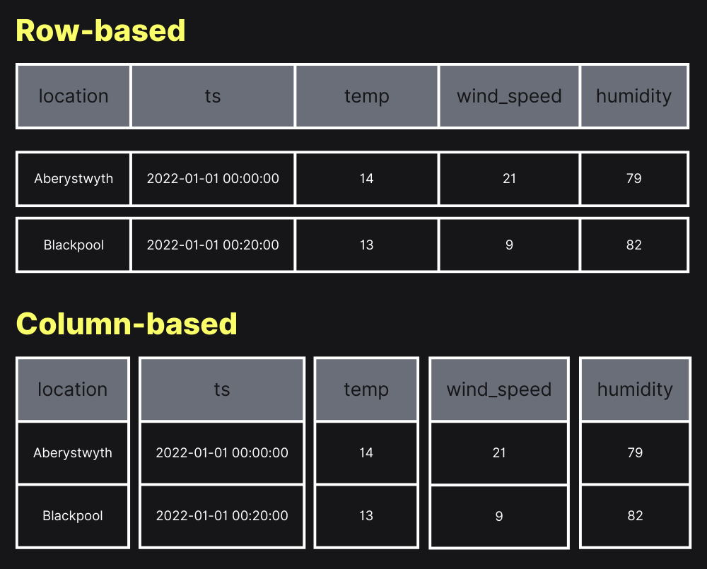
Data orientation : rows vs columns
From wikipedia: Data orientation is the representation of tabular data in a linear memory model such as in-disk or in-memory. The two most common representations are column-oriented (columnar format) and row-oriented (row format).
- row-oriented formats are more commonly used in online transaction processing (OLTP)
- column-oriented formats are more commonly used in online analytical processing (OLAP)._
Data orientation => important tradeoffs in performance and storage.
from here
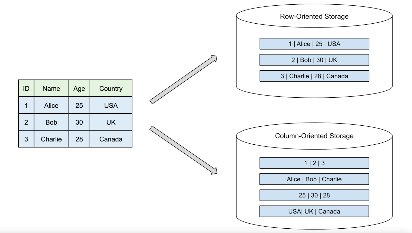
Rows orientation, storage
In a row database, how does the system know when a row ends and a new one starts ?

The database stores metadata with the data, not just the raw values.
In a row-oriented DB (e.g., PostgreSQL):
- Each row is stored as a record (tuple).
- The record has a header that includes:
- row length
- column offsets (or lengths)
- type info comes from the table schema
The DB stores rows inside pages (e.g., 8 KB in PostgreSQL).
- When reading, the system uses:
- Schema to know the order & types of columns,
- Header metadata to know where each row begins and ends.
So even if data looks like:
id, name, age, city
1, Alice, 30, New York
2, Bob, 25, Boston
On disk it’s more like:
[row header][ID][Name length][Name][Age][City length][City]
[row header][ID][Name length][Name][Age][City length][City]
The row header + schema = how the system knows where each row starts and ends.
=> easy writes; adding a new row = just add to the end of the last row
Columnar database storage
Column-based databases store data by columns instead of rows.
Each column’s values are stored together.
In a columnar system, the data is stored as (with also approriate headers):
[1, 2][Alice, Bob][30, 25][New York, Boston]
- more difficult to retrieve single rows since there are gaps between the row values,
- but column operations such as filters or aggregation are much faster than in a row-oriented database.

Columnar database in 2 mns
see also this article what is columnar database?
Comparison on simple JOIn
Let’s compare the same join query on a row database (PostgreSQL) vs a columnar database (BigQuery) and explain the difference in execution plans.
Example Schema
Two tables:
customers (customer_id, name, city)
orders    (order_id, customer_id, amount)
We want total money spent per customer:
SELECT c.name, SUM(o.amount) AS total_spent
FROM customers c
JOIN orders o
  ON c.customer_id = o.customer_id
GROUP BY c.name;
In PostgreSQL (Row-oriented)
How it executes:
- Uses indexes on
customer_idif they exist. - Reads rows directly since each row is stored together.
- Joins using nested loop or hash join, depending on table size.
Execution behavior:
Fetch row from customers → Lookup matching rows in orders using index → Aggregate
- ✔️ Fast when few customers or selective index filters.
- ✔️ Great for OLTP queries hitting a few rows at a time.
- ❌ Slower when tables become very large (millions+) → needs scaling.
In BigQuery (Columnar / Distributed Engine)
How it executes:
- Columns stored separately: reads only
customer_id,name, andamount. - Performs a distributed hash join across many workers.
- Uses column pruning (only reads necessary columns) + compression to reduce volume of data scanned.
- If one table is small (e.g., customers), it broadcasts it to all nodes.
Execution style:
Scan columnar segments → Build distributed hash table → Parallel join → Parallel aggregate
- ✔️ Very fast on huge datasets (billions of rows).
- ✔️ Scales automatically.
- ❌ Inefficient for queries touching only a few individual rows (no indexes).
Massively parallel
BigQuery is massively parallel because both the data and the query execution are distributed across many machines working at the same time.
- Data in BigQuery is stored in many chunks across distributed storage.
- When you run a query, BigQuery creates many workers (compute nodes).
- Each worker scans only its chunk of the data.
- All workers operate in parallel.
- Their partial results are then combined at the end.
So instead of one computer doing all the work
hundreds or thousands do small parts at once → massively parallel
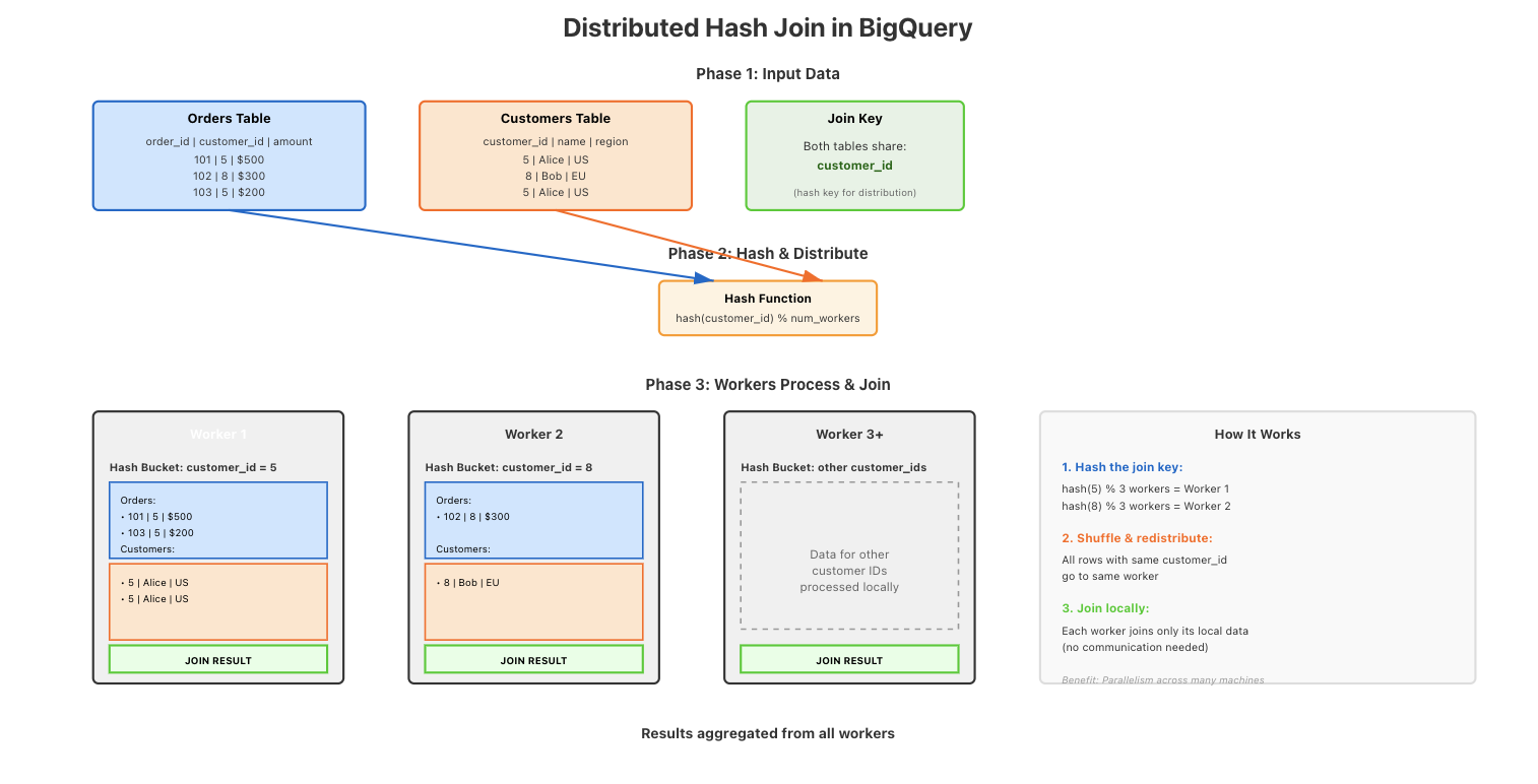
Distributed hash joins
A distributed hash join means BigQuery splits the data across many machines.
Each machine:
- Hashes the join key (e.g., customer_id).
- Sends rows with the same hash to the same worker.
- Take the customer_id → run a hash function → result decides which worker gets the row.
- That worker joins only the matching rows it received.
Hashing ensures that matching rows from two tables go to the same machine, so the join can be done in parallel.
We hash the join key to keep the workload evenly distributed across all workers and avoid hotspots: highly imbalanced workload distributions.
Example
SELECT  u.user_id, u.name, u.email, o.order_id, o.order_date
FROM    users u
JOIN    orders o ON u.user_id = o.user_id
WHERE   u.age > 18;
Shuffling Phase: BigQuery partitions both tables (users and orders) based on the join key (user_id). Each worker node processes a subset of the data, hashing the join key to distribute rows across nodes.
Build Phase: The smaller table (e.g., users) is loaded into a hash table in memory on each worker node. If the table is too large, BigQuery spills the hash table to disk.
Probe Phase: The larger table (e.g., orders) is scanned. For each row in orders, BigQuery probes the hash table to find matching rows from users using the join key (user_id). Matches are combined into the result set.
Filtering: The WHERE clause (age > 18) is applied before or during the join, depending on the query plan, to reduce the amount of data processed.
Key Points
- Automatic Optimization: BigQuery chooses the join strategy (hash, sort-merge, or broadcast) based on table size and statistics.
- Distributed Execution: The join is parallelized across multiple worker nodes for scalability.
- Efficiency: Hash joins are optimal for large datasets because they minimize data movement and leverage in-memory processing.
But why hash ?
Why not distribute the workload across workers based on the values of the key ?
1. Uniform Distribution
- Problem with Raw Values: If you distribute rows based on the raw value of the join key (e.g.,
user_id), the distribution might be skewed. Some worker nodes will receive significantly more data than others, leading to uneven workloads and slower query performance. - Hashing Solves This: A hash function (e.g.,
SHA-256or a simpler internal hash) converts the join key into a uniformly distributed integer. This ensures that rows are evenly distributed across worker nodes, balancing the load.
with Distributed hash joins
The key based load distribution is no longer based on the values of the join key
if users 1-100 have lots of orders then the worker for this range of values will be overloaded
but with hashing, head id in 1 to 100 is a unique hash and gets distributed across several workers
However, if a single key (e.g., user_id = 1) has too many rows, even hashing won’t help—one worker will still be overloaded.
2. Avoiding Hotspots
- Example Without Hashing:
If
user_idvalues are sequential (1, 2, 3, ...), and you distribute them by value ranges (e.g., Node 1 gets 1-1000, Node 2 gets 1001-2000, etc.), a few nodes might end up processing most of the data if the keys are not uniformly distributed. - With Hashing: The hash function maps similar keys (e.g., 1, 2, 3) to random-looking integers, ensuring that rows with similar keys are spread across different nodes. This prevents any single node from becoming a bottleneck.
3. Efficient Lookup
- Hash Tables:
During the build phase, the smaller table is loaded into a hash table on each worker node. The hash of the join key is used as the index for fast lookups during the probe phase.
- Without hashing, you’d need a more complex indexing mechanism (e.g., a sorted list or B-tree), which is slower for in-memory operations.
- O(1) Lookup Time: Hash tables provide constant-time lookups, making the join operation much faster compared to linear scans or binary searches.
4. Handling Large Datasets
-
Partitioning: Hashing allows BigQuery to partition the data into smaller chunks that can be processed independently by different workers. This is critical for distributed systems where data is too large to fit on a single machine.
-
Minimizing Data Movement: By hashing the join key, each worker only needs to communicate with other workers handling the same hash bucket, reducing network overhead.
What Happens If You Don’t Hash?
- Skewed Workloads: Some workers might process significantly more data than others, leading to stragglers that slow down the entire query.
- Inefficient Joins: Without hashing, you’d need to broadcast one table to all workers (for small tables) or use a sort-merge join, which requires sorting both tables and is more expensive for large datasets.
Summary
Hashing the join key ensures:
- Balanced workloads across workers.
- Fast lookups using hash tables.
- Minimal data movement during the join.
- Scalability for large datasets.
BigQuery (and other distributed databases) use hashing because it’s the most efficient way to distribute and join data in parallel.


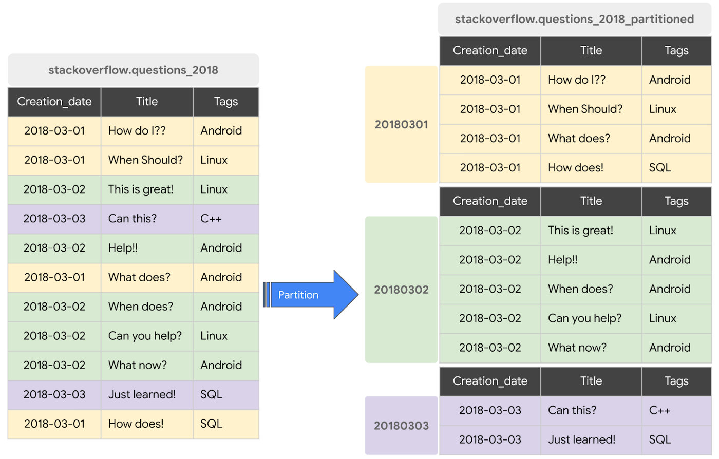
Partitioning
Columnar orientation splits the data with respect to columns width / column reduction. The engine only looks up the columns it needs
BQ has a 2nd level of data reduction: partitionning which is height / row reduction
Partitioning
Partitioning is splitting a large table into smaller chunks (partitions) based on a granular column — usually date, timestamp, or integer range.
Instead of scanning the whole table, BigQuery will only scan the partitions needed for the query.
- 2024-01-01 → partition
- 2024-01-02 → partition
- 2024-01-03 → partition
The query
SELECT * FROM events
WHERE event_date = "2024-01-02";
→ BigQuery reads only the 2024-01-02 partition, not the entire table.
/data/2024-01-01/ (rows for Jan 1, 2024)
/data/2024-01-02/ (rows for Jan 2, 2024)
...
Why it matters:
- Row-level pruning: If your query filters on the partition column (e.g., WHERE date = '2024-01-01'), BigQuery only reads the relevant partition, skipping the rest.
- Cost savings: Fewer rows scanned = lower compute costs and faster queries.
SELECT name, age
FROM users
WHERE date = '2023-01-01';
- Columnar: Only the name and age columns are read (ignoring email, user_id, etc.).
- Partitioning: Only the rows in the date = '2023-01-01' partition are scanned.
How to create a table with partionning
CREATE TABLE project.dataset.orders (
  order_id INT64,
  customer_id INT64,
  order_date DATE,
  amount FLOAT64
)
PARTITION BY DATE(order_date);
Or with extra clustering
CREATE TABLE project.dataset.customer_orders (
  order_id INT64,
  customer_id INT64,
  order_date DATE,
  region STRING,
  amount FLOAT64
)
PARTITION BY DATE(order_date)
CLUSTER BY customer_id, region;
Cluster by
CLUSTER BY further organizes the data within each partition into physical chunks.
Without clustering:
Partition: 2025-01-01
├── All rows for that date stored together
└── Mixed customer_ids and regions scattered throughout
With clustering:
Partition: 2025-01-01
├── Cluster 1: customer_id 1-100, region "US"
├── Cluster 2: customer_id 1-100, region "EU"
├── Cluster 3: customer_id 101-200, region "US"
└── Cluster 4: customer_id 101-200, region "EU"
The Physical Storage Benefit
When you query with a filter like:
SELECT * FROM customer_orders
WHERE DATE(order_date) = '2025-01-01'
  AND customer_id = 50
  AND region = 'US';
BigQuery does this:
- Partition pruning: Only reads the 2025-01-01 partition (skips all other dates)
- Cluster pruning: Within that partition, only reads Cluster 1 & 2 (skips clusters with customer_id > 100)
- Region pruning: Further narrows to just the "US" cluster
This dramatically reduces the amount of data read from disk. you're scanning maybe 5-10% of the partition instead of 100%.
Key Point
Clustering creates sort order within the partition files. It doesn't create separate sub-partitions you can see; it's transparent internal organization.
But the physical data is ordered so that:
- Related rows (same customer_id, same region) are stored adjacently on disk
- BigQuery's statistics know which file chunks contain which values
- Unnecessary file chunks can be skipped during queries
No indexing needed
-> Partitioning and Clustering Replace Indexes
BigQuery does not support manual indexes because its architecture (columnar + partitioning + clustering) makes them unnecessary for most analytical queries. Design your tables with partitioning/clustering to optimize performance.
Recap
So partitioning is subseting a table wrt to rows while columnar data organization is subsetting a table wrt to columns.
- Columnar reduces width scanned.
- Partitioning + clustering reduces height scanned.
When you run a query:
SELECT col1, col3
FROM my_table
WHERE date = '2024-01-02';
BigQuery does this:
- Identify only the partition for
2024-01-02→ ignore all other row groups. - Inside that partition, read only col1 and col3 → ignore all other columns.
- Reassemble just those columns using row index alignment.
| Step | What is filtered | Effect |
|---|---|---|
| 1. Partition pruning | Rows | Skip irrelevant row blocks |
| 2. Column pruning | Columns | Skip irrelevant columns |
| 3. Join columns back | Based on row index | Reconstruct the requested rows |
Partitioning removes rows you don’t need, columnar storage skips columns you don’t need. -> BQ can handle super large datasets
but it's not the only thing
- Distributed Storage + Compute Separation
- Data lives in Colossus (Google’s distributed file system).
- Compute nodes don’t store data → they pull only what they need.
- Lets BigQuery scale compute independently of storage.
- Massively Parallel Processing (MPP)
- A query is broken into many small tasks.
- Tasks run in parallel across many machines.
- More data → more workers → performance stays high.
- Data Locality & Sharding
- Large tables are automatically sharded into chunks.
- Workers process chunks close to where they are stored, reducing network cost.
- Compression + Encodings
Columns often contain similar values → BigQuery applies:
- Dictionary encoding
- Run-length encoding
- Delta encoding
Smaller data → lower scan cost → faster reads.
- Broadcast + Distributed Hash Joins
Small tables are broadcast to all workers. : it is faster to copy the small table to every worker machine. Broadcasting means BigQuery copies the small table to all workers so each worker can join locally without moving large data around.
Large tables are joined in parallel using hash partitioning.
PostgreSQL performance is mainly about:
- Indexes → quickly find specific rows.
- Query planner / optimizer → choose best join + access strategy.
- Caching → keep hot data in RAM.
- Single-node execution → scale by using a bigger server.
Optimized for many small, precise lookups.
BigQuery performance is mainly about:
-
Subsetting the data before processing:
- Columnar storage → read only needed columns
- Partitioning → read only needed row ranges
- Further clustering → break partitions into parallel chunks
-
Massively parallel execution across many workers
-
Broadcast / distributed hash joins
-
Vectorized execution + compression
Optimized for large scans and aggregations.
PostgreSQL goes fast by finding the right rows efficiently;
BigQuery goes fast by processing huge amounts of data in parallel while skipping everything it doesn’t need.
the user-facing SQL looks the same, but the execution model underneath is completely different.
You can write:
SELECT city, AVG(amount)
FROM orders
GROUP BY city;
This works in PostgreSQL and BigQuery.
But the engines behave differently
| Database | How it executes the SQL | What it's optimized for |
|---|---|---|
| PostgreSQL | Uses indexes, row-level access, and a single-machine query planner | Fast small lookups and transactions |
| BigQuery | Skips columns, skips partitions, shards data, and runs work in parallel on many machines | Fast large scans and aggregations |
Machine Learning in BQ
BigQuery ML: Machine Learning in SQL
- Train and deploy ML models directly in BigQuery using standard SQL.
- Key benefit: No data movement, no infrastructure setup, and no need for external tools.
- Use cases: Predictive analytics, classification, regression, clustering, time series forecasting, and anomaly detection.
How It Works
- Data Preparation: Store your dataset in a BigQuery table.
- Model Training: Use
CREATE MODELwith SQL to train models. - Evaluation: Assess model performance with
ML.EVALUATE. - Prediction: Generate predictions using
ML.PREDICT. - Integration: Embed models in queries, dashboards, or workflows.
Training a Model
-- Example: Logistic Regression
CREATE OR REPLACE MODEL `mydataset.my_model`
OPTIONS(
  model_type='LOGISTIC_REG',
  input_label_cols=['label']
) AS
SELECT * FROM `mydataset.training_data`;
- Supported Models:
LINEAR_REG(Regression)LOGISTIC_REG(Classification)KMEANS(Clustering)ARIMA_PLUS(Time Series)AUTOML_CLASSIFIER/AUTOML_REGRESSOR(AutoML)
Evaluating and Predicting
- Evaluate:
SELECT * FROM ML.EVALUATE(MODEL `mydataset.my_model`); - Predict:
SELECT * FROM ML.PREDICT(MODEL `mydataset.my_model`, TABLE `mydataset.new_data`);
Key Features
- Serverless: No infrastructure to manage.
- Scalable: Automatically handles large datasets.
- Cost-effective: Pay only for queries and storage.
- Accessible: SQL interface for analysts and data scientists.
- Integration: Works seamlessly with BigQuery tables and Google Cloud services.
Use Cases
- Customer churn prediction
- Sales forecasting
- Fraud detection
- Recommendation systems
- Anomaly detection
Advanced Options
- Hyperparameter Tuning: Customize model parameters during training.
- Import Models: Use pre-trained TensorFlow or XGBoost models.
- Export Models: Deploy models outside BigQuery if needed.