RDBMS & SQL
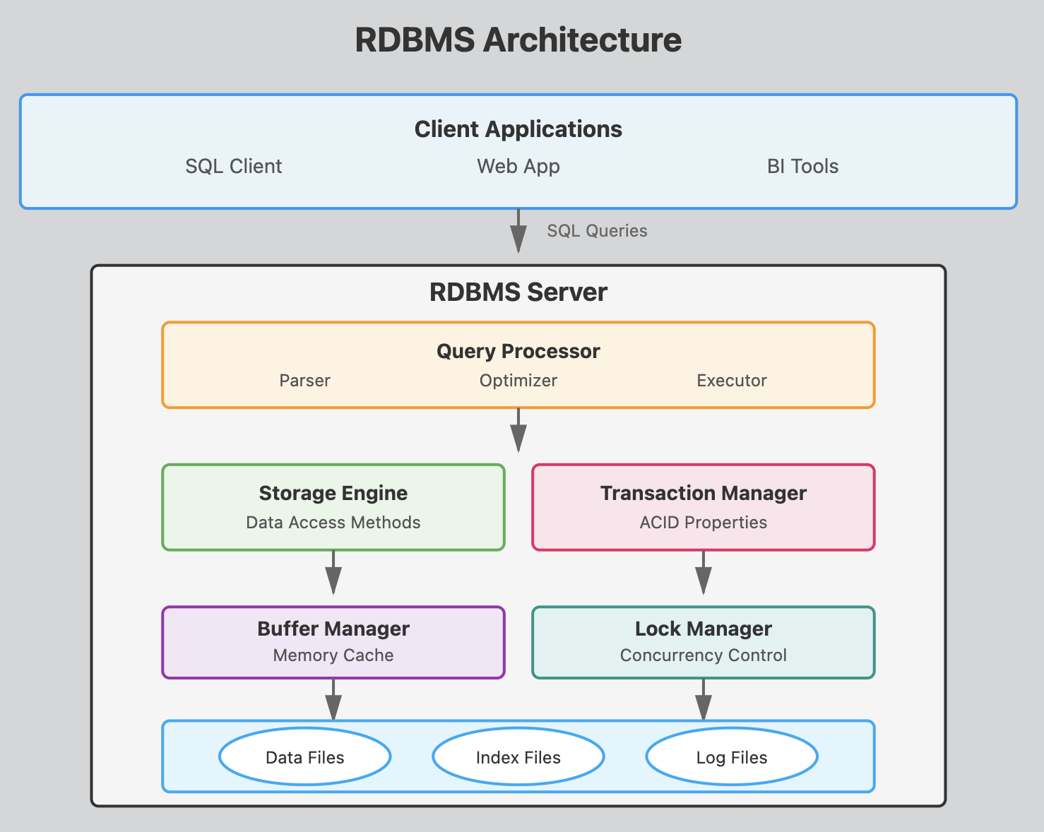
This architecture shows how a SQL query flows from the client through various processing layers before reaching the actual data on disk, with each component playing a crucial role in ensuring efficient, reliable database operations.
RDBMS Components
Client Applications Layer
SQL Clients, Web Apps, BI Tools
These are the programs that users interact with to send SQL queries to the database. They connect to the RDBMS server using protocols like JDBC, ODBC, or native database drivers. (python, nodejs, Java, etc)
Query Processor
- Parser
Checks SQL syntax and converts queries into an internal format the database can understand. It validates that tables and columns exist and that the user has proper permissions.
- Optimizer
Determines the most efficient way to execute a query by analyzing different execution plans. It considers factors like available indexes, table statistics, and join methods to minimize resource usage. This is what makes Postgresql super efficient.
- Executor
Carries out the optimized query plan by coordinating with other components to retrieve or modify data according to the SQL command.
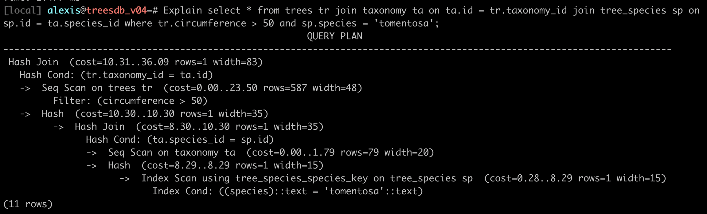
Example of a query plan with EXPLAIN
Explain
SELECT * FROM trees tr
JOIN taxonomy ta on ta.id = tr.taxonomy_id
JOIN tree_species sp on sp.id = ta.species_id
WHERE tr.circumference > 50 and sp.species = 'tomentosa';
Storage Engine
- Data Access Methods
Manages how data is physically stored and retrieved from disk.
It handles different storage structures like heap files, B-trees for indexes, and implements algorithms for efficient data access.

Transaction Manager
- ACID Properties
Ensures database transactions are
- Atomic: all-or-nothing
- Consistent: maintains data integrity
- Isolated: concurrent transactions don’t interfere
- Durable: committed changes persist even after system failures
Buffer Manager
Memory Cache
- Keeps frequently accessed data pages in RAM to reduce disk I/O.
- Manages the buffer pool using replacement algorithms like LRU (Least Recently Used) when memory is full.
Lock Manager
Concurrency Control
- Coordinates multiple users accessing the database simultaneously by managing locks on data.
- Prevents conflicts and ensures transaction isolation through various locking protocols.
Database Files
-
Data Files - Store the actual table records and rows containing your business data.
-
Index Files - Contain sorted pointers to data locations, speeding up queries by avoiding full table scans.
-
Log Files - Record all database changes for recovery purposes, allowing the system to restore data after crashes or rollback uncommitted transactions.
Components

Component families and tools
Data Manipulation:
- Internal (SQL)
The primary language for interacting with the database from within. Users and applications use SQL commands (SELECT, INSERT, UPDATE, DELETE) to query and modify data directly.
- External (Import/Export)
Tools and utilities for moving data in and out of the database. This includes bulk loading tools, data migration utilities, and export functions for backing up or transferring data to other systems.
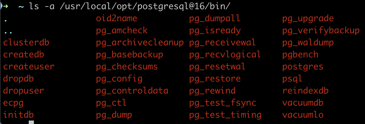
in Postgres
In postgresql we have command line executables: createdb, dropdb, pg_dump, pg_restore, pg_dumpall, pg_restoreall
these utilities are in the same folder as your
psqlexecutable
Database Exploitation
Organization and Optimization
Administrative functions that maintain database performance. This involves organizing data structures, managing storage allocation, and optimizing query execution paths to ensure fast response times.
In postgresql , we have for instance
Autovacuumreclaims storage space by cleaning up deleted/updated rowsTOAST(oversized attribute storage) manages large field values.VACUUM/REINDEX/CLUSTER: Manual commands to reorganize data and indexes for better performance.
Core Components
-
SQL Layer - The query processing interface that interprets SQL commands, validates syntax, checks permissions, and translates high-level queries into low-level operations the database engine can execute.
-
Compacting and Cold Recovery - Maintenance operations that reclaim unused space (compacting) and restore the database from backups or after unexpected shutdowns (cold recovery). These ensure data integrity and efficient storage usage.
-
Database Core (Tables, Views, Index)
The logical database structure:
- Tables: Store actual data in rows and columns
- Views: Virtual tables created from queries that provide customized data presentations
- Indexes: Sorted data structures that speed up data retrieval operations
add : functions, triggers, sequences, etc
File System Layer
NTFS, NFS, etc. - The underlying operating system file systems where database files are physically stored. The database management system interfaces with these file systems to read and write data to disk. Common examples include:
- ext4 (Linux)
- NFS (Network File System for Unix/Linux)
- APFS (macOS)
- NTFS (Windows)
![]()
Why Learn SQL in 2025?
- Universal: Every database speaks SQL
- Stable: Skills last your entire career
- Powerful: Complex operations in few lines
- Required: Every tech job posting mentions it
- Gateway: Opens doors to data science, analytics, engineering
Master SQL, and you’ll never lack job opportunities
SQL
- created 1970s, standard (ANSI, ISO) since 1986
- declarative language
- composed of sub languages / modules
- implementations varies across vendors

Evolution since the 1970s
SQL was created in the early 1970s. Here are the major features added through its evolution:
SQL-86 (SQL-87) - First ANSI Standard
- Basic SELECT, INSERT, UPDATE, DELETE operations
- Simple JOIN syntax
- Basic data types (INTEGER, CHAR, VARCHAR)
SQL-89 (SQL1)
- Integrity constraints (PRIMARY KEY, FOREIGN KEY)
- Basic referential integrity
SQL-92 (SQL2)
- New data types (DATE, TIME, TIMESTAMP, INTERVAL)
- Outer joins (LEFT, RIGHT, FULL)
- CASE expressions
- CAST function for type conversion
- Support for dynamic SQL
SQL:1999 (SQL3)
- Regular expressions
- Object-oriented features (user-defined types, methods)
- Array data types
- Window functions (ROW_NUMBER, RANK)
- Common Table Expressions (WITH clause)
SQL:2003
- XML data type and functions
- MERGE statement (UPSERT)
- Auto-generated values (IDENTITY, sequences)
- Standardized window functions
SQL:2006
- Enhanced XML support
- XQuery integration
- Methods for storing and retrieving XML
SQL:2008
- TRUNCATE statement
- INSTEAD OF triggers
- Enhanced MERGE capabilities
SQL:2011
- Temporal databases (system-versioned tables)
- Enhanced window functions
- Improvements to CTEs
SQL:2016
- JSON support (JSON data type and functions)
- Row pattern recognition
SQL:2023 (Latest)
- SQL/PGQ (Property Graph Queries)
- Multi-dimensional arrays
- More JSON features
- Graph database capabilities
Why SQL Survived 50 Years
# Python changes every few years
print "Hello"     # Python 2 (dead)
print("Hello")    # Python 3

# JavaScript changes constantly
var x = 5;        // Old way
let x = 5;        // New way
const x = 5;      // Newer way
-- SQL from 1990s still works today!
SELECT * FROM users WHERE age > 18;
SQL is the COBOL that actually stayed relevant
SQL vs Programming Languages
Imperative (Python/Java/C++): “HOW to do it”
results = []
for user in users:
    if user.age > 21 and user.country == 'France':
        results.append(user.name)
return sorted(results)
Declarative (SQL): “WHAT you want”
You describe the result, the database figures out HOW
Declarative means you describe what you want, not how to do it.
In SQL, you state the result you want, and the database (query planner) figures out how to get it.
SELECT name FROM students WHERE grade > 15;
- You declare: “Give me the names of students with grade > 15.”
- You don’t say: “Go through each student row, check grade, and collect names.”
✅ You focus on what, not how — that’s why SQL is declarative.
SQL + Modern Tools
SQL isn’t just for database admins anymore:
- Data Scientists: SQL + Python/R
- Analysts: SQL + Tableau/PowerBI
- Engineers: SQL + ORMs
- Product Managers: SQL + Metabase
- Machine Learning: SQL + Feature stores
# Modern data stack
df = pd.read_sql("SELECT * FROM events WHERE date > '2024-01-01'", conn)
model.train(df)
SQL Dialects
Same Language, Different Accents
| Standard SQL | PostgreSQL | MySQL | SQL Server |
|---|---|---|---|
SUBSTRING() |
SUBSTRING() |
SUBSTRING() |
SUBSTRING() |
| ❌ | LIMIT 10 |
LIMIT 10 |
TOP 10 |
| ❌ | STRING_AGG() |
GROUP_CONCAT() |
STRING_AGG() |
| ❌ | ::TEXT |
❌ | CAST AS VARCHAR |
Core SQL (90%) is identical everywhere Fancy features (10%) vary
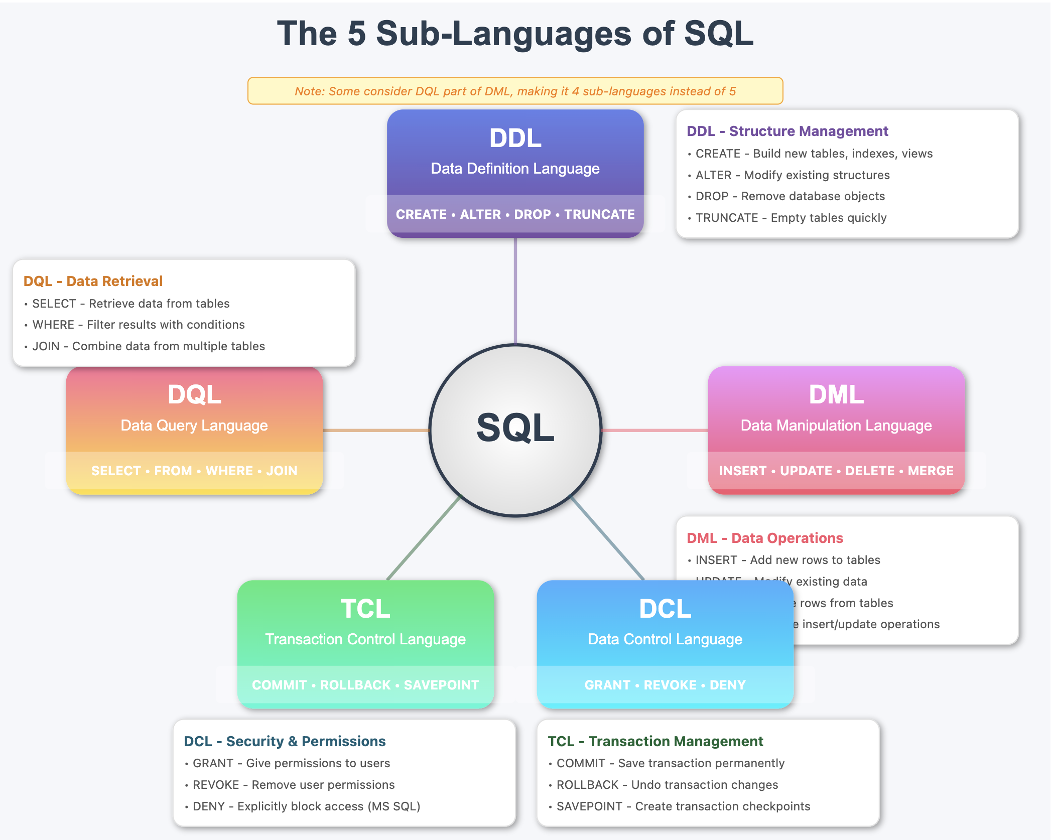
The SQL Family Tree
SQL
├── DDL (Data Definition Language)
│   └── CREATE, ALTER, DROP
├── DML (Data Manipulation Language)
│   └── INSERT, UPDATE, DELETE
├── DQL (Data Query Language)
│   └── SELECT, FROM, WHERE, JOIN
├── DCL (Data Control Language)
│   └── GRANT, REVOKE
└── TCL (Transaction Control Language)
    └── COMMIT, ROLLBACK, BEGIN
You’ll use DML and DQL 90% of the time
Some database texts combine DQL with DML since
SELECTstatements can be considered data manipulation, resulting in 4 sub-languages instead of 5.
1. DDL - Data Definition Language
Defines and manages database structure
- CREATE: Builds new database objects (tables, indexes, views, schemas)
- ALTER: Modifies existing structures (add/drop columns, change data types)
- DROP: Permanently removes database objects
CREATE
create database epitadb;
create table students (
    id serial primary key,
    name varchar(100) not null,
    age int not null,
    grade int not null
);
ALTER table students ADD COLUMN graduation_year int;
DROP table students;
Simple version
CREATE TABLE <table_name> (
    id serial primary key,
    <column_name> <data_type> <constraints>,
    <column_name> <data_type> <constraints>,
    <column_name> <data_type> <constraints>,
    <column_name> <data_type> <constraints>,
);
with index and keys:
CREATE TABLE <table_name> (
    id serial primary key,
    <column_name> <data_type> <constraints>,
    <column_name> <data_type> <constraints>,
    <column_name> <data_type> <constraints>,
    <column_name> <data_type> <constraints>,
    INDEX <index_name> (<column_name>),
    UNIQUE INDEX <index_name> (<column_name>),
    FOREIGN KEY (<column_name>) REFERENCES <table_name>(<column_name>),
);
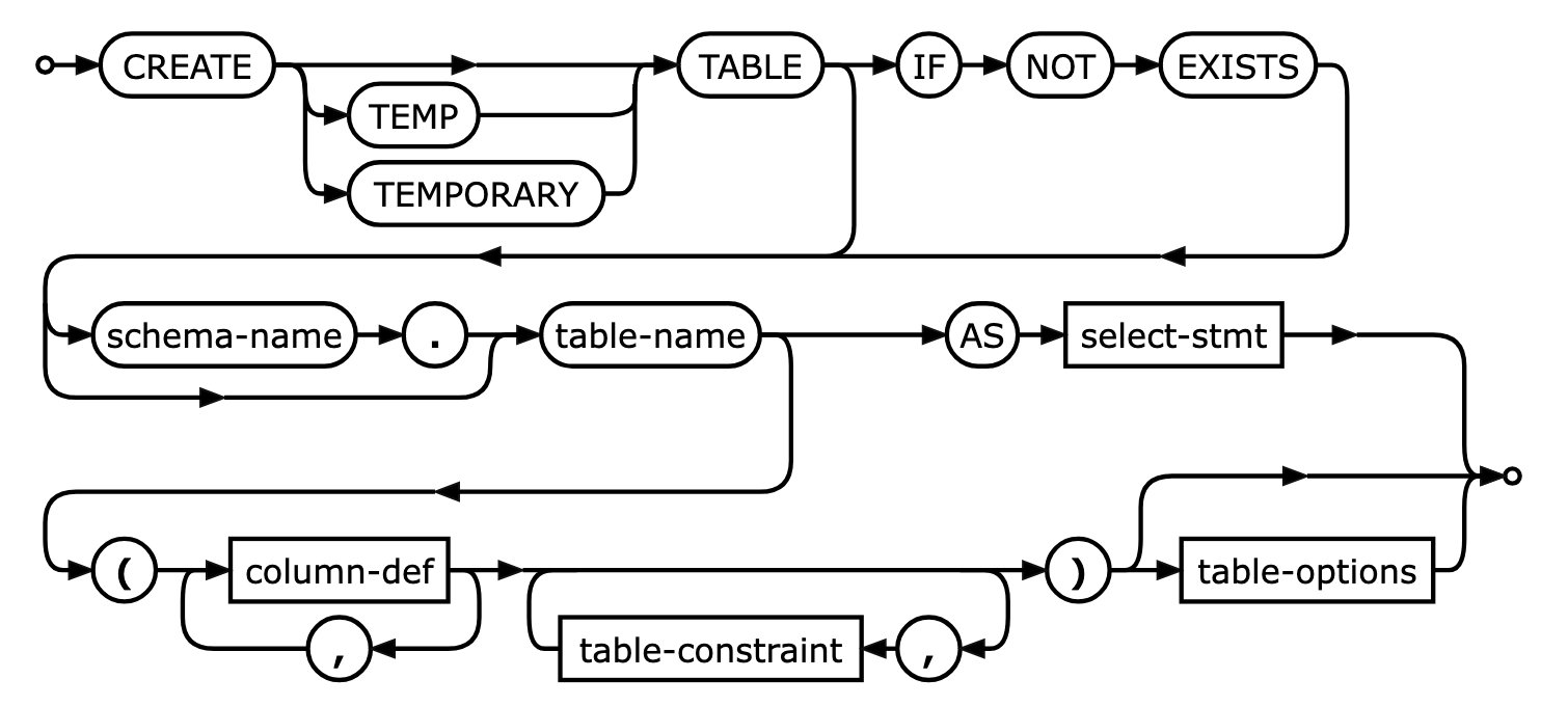
Create table documentation
Let’s look at the postgresql documentation for the create table statement:
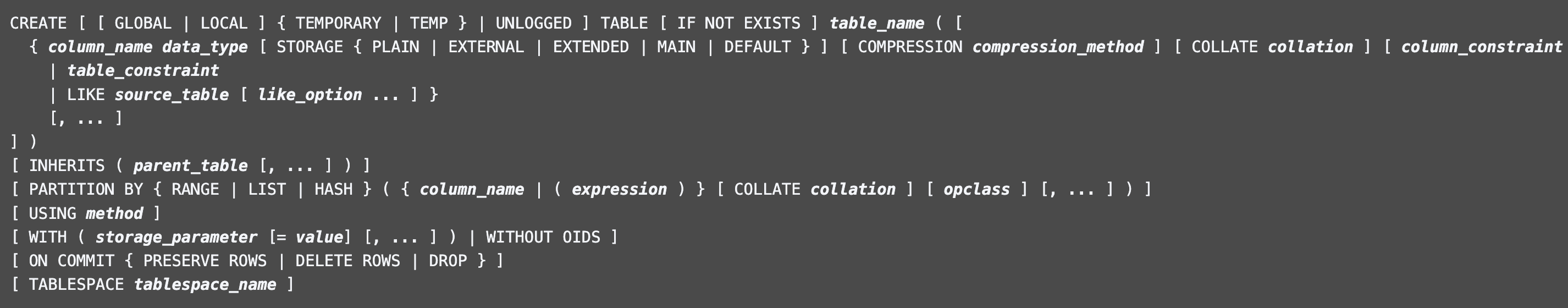
https://www.postgresql.org/docs/current/sql-createtable.html
Create table
in postgresql
CREATE TABLE employees (
    id SERIAL PRIMARY KEY,
    first_name VARCHAR(50) NOT NULL,
    last_name VARCHAR(50) NOT NULL,
    email VARCHAR(100) UNIQUE NOT NULL,
    hire_date DATE NOT NULL,
    salary NUMERIC(10, 2) NOT NULL,
    department_id INT NOT NULL,
    created_at TIMESTAMP DEFAULT CURRENT_TIMESTAMP,
    updated_at TIMESTAMP DEFAULT CURRENT_TIMESTAMP
);
It is good practice to use default values for date time columns and always have for tracabiliy purposess the 2 colums:
created_atupdated_at
attention, the last column does not have a comma
2. DML - Data Manipulation Language
Manages data within tables
- INSERT: Adds new rows of data to tables
- UPDATE: Modifies existing data values in rows
- DELETE: Removes specific rows from tables
- MERGE: Performs “upsert” operations: insert or update based on conditions
Also in DQL
Aggregate Functions (DQL)
COUNT(),SUM(),AVG(),MAX(),MIN()- Used with
GROUP BYfor summarizing data
Scalar Functions (DQL)
COALESCE()- Handles NULL valuesCAST() / CONVERT()- Type conversionSUBSTRING(), CONCAT(), TRIM()- String manipulationDATEADD(), DATEDIFF()- Date operationsROUND(), FLOOR(), CEILING()- Math functions
Clauses & Operations (DQL)
GROUP BY- Groups rows for aggregationHAVING- Filters grouped resultsORDER BY- Sorts result setsDISTINCT- Removes duplicatesUNION/INTERSECT/EXCEPT- Set operations
Window Functions (DQL)
ROW_NUMBER(),RANK(),DENSE_RANK()LAG(),LEAD()- Access other rows- Running totals and moving averages
Conditional Logic (DQL)
CASE WHEN- Conditional expressions
Insert
INSERT INTO <table_name> (
  <column_name>,
  <column_name>,
  <column_name>
)
VALUES (
  <value>,
  <value>,
  <value>
);
for instance
INSERT INTO courses (
    title,
    description,
    semester,
    hours
)
VALUES (
  "intro to databse",
  "the best database course in the universe ",
  "fall 2025",
  123
);
- the
idprimary key, gets auto-incremented - default values are applied so you do not have to specify all columns in the insert statement
- if no default values, the column will be set to
NULL
make sure
- data type match : you cannot insert an TEXT into a INT columns
- constraints will throw errors if not respected (unicity, foreign keys, etc )
Multiple rows
you can insert multiple rows in one query
INSERT INTO <table_name> (
  <column_name>,
  <column_name>,
  <column_name>
)
VALUES
  (<value>, <value>, <value>),
  (<value>, <value>, <value>),
  (<value>, <value>, <value>);
Update
UPDATE <table_name>
SET <column_name> = <value>,
  <column_name> = <value>
WHERE <condition>;
for instance:
UPDATE courses
SET title = "intro to databse",
    description = "the best intro to database course in the universe",
    semester = "fall 2025",
    hours = 4
WHERE id = 1;
3. DQL - Data Query Language
Retrieves data from the database
- SELECT: Fetches data from one or more tables
- FROM: Specifies source tables
- WHERE: Filters results based on conditions
- JOIN: Combines rows from multiple tables
SELECT <column_name>, <column_name>
FROM <table_name>
WHERE <condition>;
for instance:
SELECT title, description
FROM courses
WHERE semester = "fall 2025";
joining on the teacher id:
SELECT title, description, teachers.name
FROM courses
JOIN teachers ON courses.teacher_id = teachers.id
WHERE semester = "fall 2025";
4. DCL - Data Control Language
Controls access and permissions
- GRANT: Gives specific privileges to users/roles
- REVOKE: Removes previously granted privileges
- DENY: Explicitly prevents access (Microsoft SQL Server specific)
GRANT SELECT, INSERT, UPDATE, DELETE ON <table_name> TO <user_name>;
for instance:
GRANT SELECT, INSERT, UPDATE, DELETE ON courses TO Alexis;
DCL vs pg_hba.conf
GRANT does not modify pg_hba.conf
These control different layers of access:
pg_hba.conf (Connection Level)
- Controls WHO can connect to the server
- Controls HOW they authenticate (password, trust, etc.)
- Controls WHERE they can connect from (IP addresses)
- “Can you get in the door?”
GRANT (Permission Level)
- Controls what users can DO once connected
- Controls access to specific databases, tables, schemas
- Controls operations: SELECT, INSERT, UPDATE, DELETE, etc.
- “What can you do once you’re inside?”
Example flow:
- User tries to connect → pg_hba.conf checks if allowed
- User enters password → pg_hba.conf authentication method
- User runs
SELECT * FROM products→ GRANT checks if they have SELECT permission

Where GRANT info is stored:
- In system catalogs (internal PostgreSQL tables)
- View with:
\dp(table privileges) or\l(database privileges) in psql - Not in any config file
You need both: pg_hba.conf to allow connection + GRANT to allow operations!
5. TCL - Transaction Control Language
Manages database transactions
- COMMIT: Permanently saves all changes in a transaction
- ROLLBACK: Undoes all changes in current transaction
- SAVEPOINT: Sets a point within transaction to rollback to
BEGIN TRANSACTION;

-- Update all course credits by 1
UPDATE courses SET credits = credits + 1;

-- Give all teachers a 10% raise (you wish )
UPDATE teachers SET salary = salary * 1.10;

-- Check if any teacher salary is now over 20,000
IF EXISTS (SELECT 1 FROM teachers WHERE salary > 20000)
  BEGIN
      -- Something went wrong, undo everything
      ROLLBACK;
      PRINT 'Rolled back - salary too high! (for France)';
  END
ELSE
  BEGIN
      -- Everything looks good, save the changes
      COMMIT;
      PRINT 'Changes saved successfully!';
  END
Both COMMIT and ROLLBACK are “terminal” commands for a transaction.
They save/undo the work AND close the transaction in one go.
There’s no “END TRANSACTION” command in SQL.
Once you COMMIT or ROLLBACK, you’re done!
DDL: Data Definition Language
-- Create the structure
CREATE TABLE songs (
    id INTEGER PRIMARY KEY,
    title TEXT NOT NULL,
    artist TEXT NOT NULL,
    duration_seconds INTEGER,
    release_date DATE
);

-- Modify the structure
ALTER TABLE songs ADD COLUMN genre TEXT;

-- Destroy the structure
DROP TABLE songs;  -- ⚠️ Everything gone!
DML: Data Manipulation Language
The everyday SQL
-- Create: Add new data
INSERT INTO songs (title, artist, duration_seconds)
VALUES ('Flowers', 'Miley Cyrus', 200);

-- Read: Query data
SELECT title, artist FROM songs WHERE duration_seconds < 180;

-- Update: Modify existing data
UPDATE songs SET genre = 'Pop' WHERE artist = 'Taylor Swift';

-- Delete: Remove data
DELETE FROM songs WHERE release_date < '2000-01-01';
The SELECT Statement
This pattern solves the large majority of your data questions
SELECT     -- What columns?
FROM       -- What table?
JOIN       -- What other tables?
WHERE      -- What rows?
GROUP BY   -- How to group?
HAVING     -- Filter groups?
ORDER BY   -- What order?
LIMIT      -- How many?
SQL Reads Like English
-- Almost natural language
SELECT name, age
FROM students
WHERE grade > 15
ORDER BY age DESC
LIMIT 10;
Translates to: “Show me the names and ages of students with grades above 15, sorted by age (oldest first), but only the top 10”
This is why SQL survived: humans can read it
The Power of JOINs
Without JOIN (multiple queries):
# Get user
user = db.query("
  SELECT * FROM users WHERE id = 42
")
# Get their orders
orders = db.query(f"
  SELECT *
  FROM orders
  WHERE user_id = {user.id}
")
# Get order details
for order in orders:
    items = db.query(f"
      SELECT *
      FROM items
      WHERE order_id = {order.id}
    ")
With JOIN (one query):
SELECT u.name, o.date, i.product
FROM users u
JOIN orders o ON u.id = o.user_id
JOIN items i ON o.id = i.order_id
WHERE u.id = 42;
Joins
What is a JOIN?
A JOIN combines rows from two or more tables based on a related column between them.
Basic JOIN Syntax:
SELECT columns
FROM table1
JOIN table2
ON table1.column = table2.column;
- join on
keys
Example : the tree database
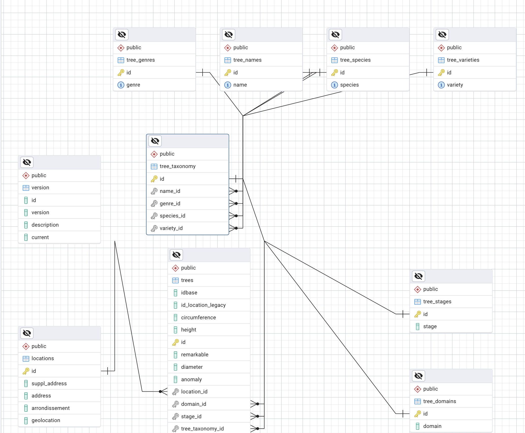
using aliases: trees : tr, taxonomy : ta, tree_species : sp
SELECT * FROM trees tr
JOIN taxonomy ta on ta.id = tr.taxonomy_id
JOIN tree_species sp on sp.id = ta.species_id
WHERE tr.circumference > 50 and sp.species = 'tomentosa';
instead of
SELECT * FROM trees
JOIN taxonomy on taxonomy.id = trees.taxonomy_id
JOIN tree_species on tree_species.id = taxonomy.species_id
WHERE trees.circumference > 50 and tree_species.species = 'tomentosa';
Types of JOINs
1. INNER JOIN (Default)
Returns only matching records from both tables.
SELECT customers.name, orders.order_date
FROM customers
INNER JOIN orders
ON customers.customer_id = orders.customer_id;
Example
- a movie table
- an actor table
- a movie can have 0 or more actors
- an actor can be in 0 or more movies
INNER JOIN
SELECT
    m.movie_id,
    m.release_year,
    m.title,
    a.actor_name,
FROM movies m
JOIN actors a ON m.movie_id = a.movie_id;
Result example:
| movie_id | title | release_year | actor_name |
|---|---|---|---|
| 1 | The Matrix | 1999 | Keanu Reeves |
| 1 | The Matrix | 1999 | Laurence F. |
| 2 | Inception | 2010 | Leonardo D. |
Movies with no actors will not be shown. NULL values are used instead:
| movie_id | title | release_year | actor_name | role |
|---|---|---|---|---|
| 3 | Documentary XYZ | 2023 | NULL | NULL |
| 4 | Silent Film | 1920 | NULL | NULL |
Similarly the actors with no movies will not be shown.
2. LEFT JOIN (LEFT OUTER JOIN)
Returns all records from the left table (the first from), and matched records from the right table (the table after the join).
SELECT
    m.movie_id,
    m.title,
    m.release_year,
    a.actor_name,
    a.role
FROM movies m
LEFT JOIN actors a ON m.movie_id = a.movie_id
ORDER BY m.title;
Result example:
also returns the movies with no actors
| movie_id | title | release_year | actor_name | role |
|---|---|---|---|---|
| 1 | The Matrix | 1999 | Keanu Reeves | Neo |
| 1 | The Matrix | 1999 | Laurence F. | Morpheus |
| 2 | Inception | 2010 | Leonardo D. | Cobb |
| 3 | Documentary XYZ | 2027 | NULL | NULL |
| 4 | Silent Film | 1920 | NULL | NULL |
The key point: LEFT JOIN keeps ALL movies, even if they have no actors in the actors table. Those movies will show NULL values for the actor columns.
This may eventually be useful for:
- Seeing all movies in your database (with or without cast info)
- Finding movies that have no actors assigned yet (like documentaries or movies with missing data)
- Making sure you don’t lose any movies from your results just because actor data is incomplete
3. RIGHT JOIN (RIGHT OUTER JOIN)
Returns all records from the right table, and matched records from the left table.
SELECT
    m.movie_id,
    m.title,
    m.release_year,
    a.actor_name,
    a.role
FROM movies m
RIGHT JOIN actors a ON m.movie_id = a.movie_id
ORDER BY m.title;
NULL values appear for actors with no movie
4. FULL OUTER JOIN
Returns all records when there’s a match in either table.
SELECT
    m.movie_id,
    m.title,
    m.release_year,
    a.actor_name,
    a.role
FROM movies m
FULL OUTER JOIN actors a ON m.movie_id = a.movie_id
ORDER BY m.title;
Result example:
All movies AND all actors, even unmatched ones
| movie_id | title | release_year | actor_name | role |
|---|---|---|---|---|
| NULL | NULL | NULL | Alphonse | NULL |
| NULL | NULL | NULL | Nephew of Alphonse | NULL |
| 1 | The Matrix | 1999 | Keanu Reeves | Neo |
| 2 | Inception | 2010 | Leonardo D. | Cobb |
| 3 | Documentary XYZ | 2023 | NULL | NULL |
| 4 | Silent Film | 1920 | NULL | NULL |
The key difference: FULL OUTER JOIN keeps EVERYTHING from both tables:
- All movies (even those with no actors)
- All actors (even those not assigned to any movie)
This creates three groups in your results:
- Matched records - Movies with their actors
- Movies with no actors - NULLs in actor columns
- Actors with no movies - NULLs in movie columns
5. CROSS JOIN
when you do not have a ON clause, it is a cross join
Returns the Cartesian product of both tables (every row paired with every row).
SELECT customers.name, products.product_name
FROM customers
CROSS JOIN products;

Performance Tips
- Always JOIN on indexed columns when possible
- Use INNER JOIN when you only need matching records
- Be careful with CROSS JOIN - can produce huge result sets
- Filter early with WHERE clauses to reduce data processing
Common Mistakes to Avoid
- Ambiguous column names (always use table prefixes)
- Forgetting the ON clause (creates a CROSS JOIN)
- Wrong JOIN type (using INNER when you need LEFT)
- Not considering NULL values in OUTER JOINs
Vocabulary
Projection
When we select a set of columns and not all the columns we are doing a projection
This returns all the columns of the table:
select * from movies
This returns only the title and released_year column
select title, released_year from movies
We can apply functions to the columns during the projections, for instance:
select avg(IMDB_Rating), max(IMDB_Rating), min(IMDB_Rating) from movies;
Filtering
When we select a set of rows and not all the rows we are doing a filtering
select title from movies where IMDB_Rating > 8;
we can use multiple conditions
select title
from movies
where IMDB_Rating > 8
AND released_year > 2000;
select title
from movies
where IMDB_Rating > 8
OR released_year > 2000;