Big Query
A serverless huge scale database from Google Cloud
- serverless
- row vs columnar database
- partitionning
Google cloud, AWS, Azure
hyper scalers: GCP, aws, azure
- very large number of services from barebones VMs to serverless platforms
- compute, databases, network, storage, security, monitoring,
Alternatives:
- [FR] OVH, scaleway, …
google cloud databases offerings
In Nov 2025, GOogle Cloud offers 12 different databases
- Cloud SQL → Managed PostgreSQL / MySQL.
- Cloud Spanner → Global, horizontally scalable SQL with strong consistency.
- Firestore / Datastore → NoSQL document store, real-time sync.
Analytical / OLAP
- BigQuery → Serverless data warehouse for large-scale analytics.
In-memory / Caching
- MemoryStore → Managed Redis / Memcached. Redis (Remote Dictionary Server) is an in-memory key–value database, used as a distributed cache and message broker, with optional durability.
Key-Value / High-throughput
- Bigtable → Wide-column NoSQL for huge time-series / IoT workloads.
to play along
- go to console.cloud.google.com
- open an account
You should have 300$ credits to begin exploring.
- Enable BigQuery API
Big Query also offers a sandbox
Handle with extreme caution
Caution: use at your own risks. It’s very easy to spin up large resouces and blow up your budget.
Do not try if you are not confortable with using cloud resources with your own credit card.
make sure you can monitor your usage consumption in Billing
turn off all resources you’ve setup.
do not publish API keys and access credentials
BQ Billing
3 tier: storage + analytical + transfer
Storage is cheap. Querying is what you pay for.
How to work with BQ
example: this will list 10 datasets from bigquery-public-data
bq ls --project_id=bigquery-public-data --max_results=10
BG public datasets : bigquery-public-data
- public
- hosted by Google for free
- pay only for the queries
- first 1 TB per month is free
BQ vs postgresql, mysql etc
BQ is:
- Serverless, fully managed — no infrastructure to manage.
- Massively parallel — scales automatically for huge datasets.
- Columnar storage + query engine optimized for analytics (OLAP).
- Best for read-heavy, large-scale analytical queries.
- Pricing based on data scanned + storage.
- Integrates tightly with GCP ecosystem and BI tools.
BQ is OLAP, postgres is OLTP
BQ is not made for heavy transactional workloads.
- BQ Queries scan large batches of data at once (columnar + MPP), not single-row updates.
- Writes are slow and done in batches, not optimized for frequent INSERT/UPDATE/DELETE.
- No row-level locking or ACID-style transaction guarantees like PostgreSQL. (Atomicity, Consistency, Isolation, and Durability,)
- Costs scale with data scanned → small frequent operations become inefficient.
In short: BigQuery = big reads, PostgreSQL = frequent small writes.
Latency vs Throughput
- latency: How fast you get one result.
-
throughput: How many results you get per second.
- Latency is higher — results are optimized for throughput, not response time.
BQ is not trying to return each query very fast.
BQ is designed to handle very large amounts of data efficiently, even if that means each individual query takes longer to start or finish.
You might wait 2–5 seconds for the first result (higher latency), but the system can process huge datasets (terabytes) in one go (high throughput).
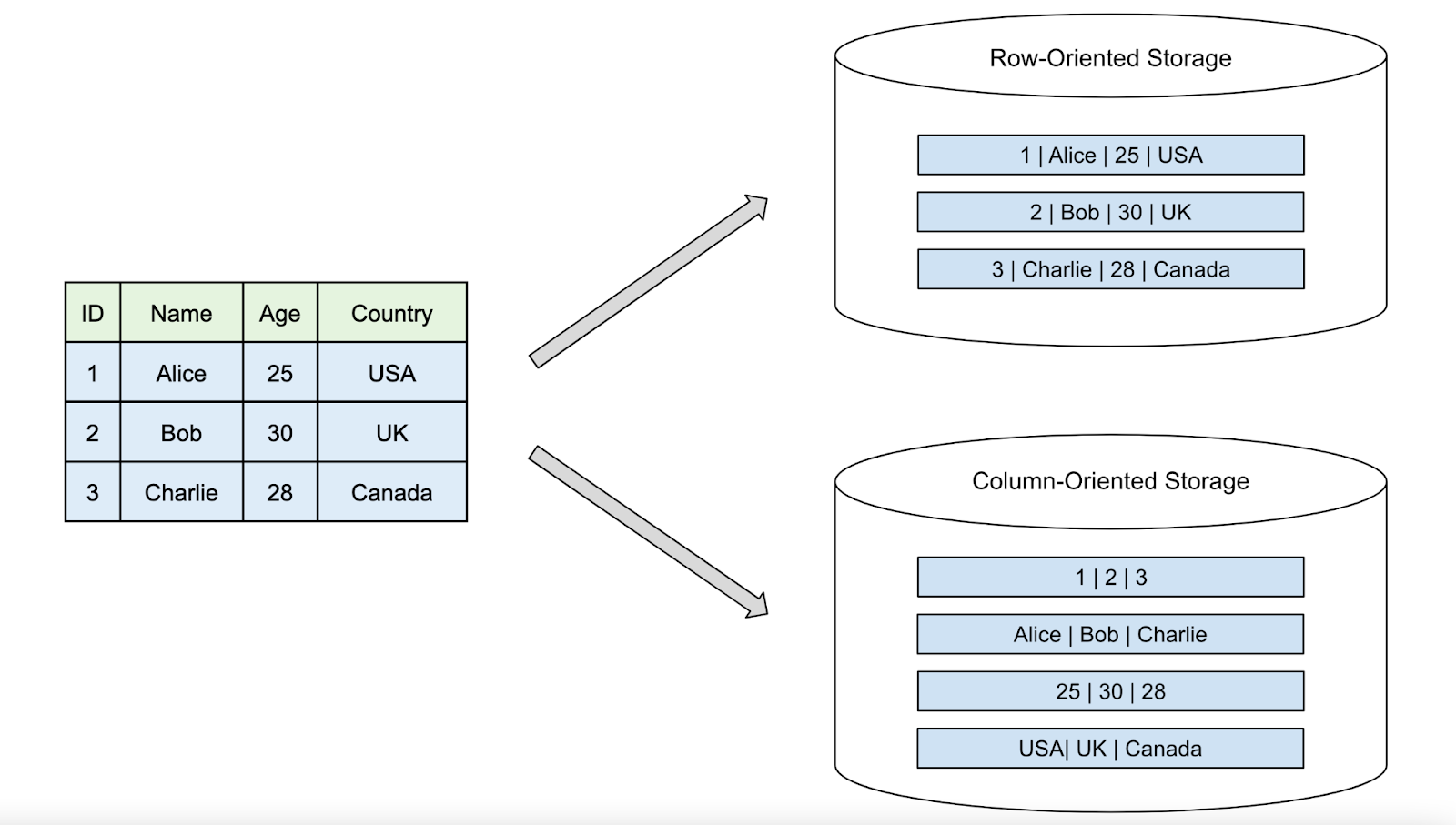
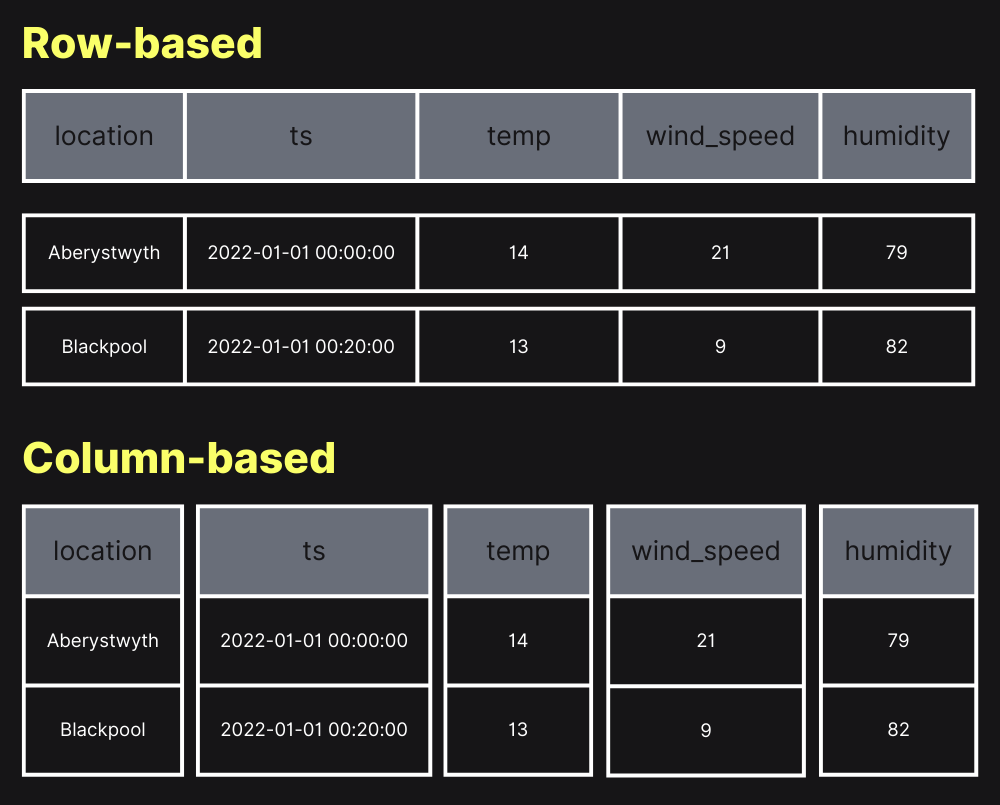
Data orientation : rows vs columns
From wikipedia: Data orientation is the representation of tabular data in a linear memory model such as in-disk or in-memory. The two most common representations are column-oriented (columnar format) and row-oriented (row format).
- row-oriented formats are more commonly used in online transaction processing (OLTP)
- column-oriented formats are more commonly used in online analytical processing (OLAP)._
Data orientation => important tradeoffs in performance and storage.
 from here
Rows orientation, storage
In a row database, how does the system know when a row ends and a new one starts ?

The database stores metadata with the data, not just the raw values. In a row-oriented DB (e.g., PostgreSQL):
- Each row is stored as a record (tuple).
- The record has a header that includes:
- row length
- column offsets (or lengths)
- type info comes from the table schema
The DB stores rows inside pages (e.g., 8 KB in PostgreSQL).
- When reading, the system uses:
- Schema to know the order & types of columns,
- Header metadata to know where each row begins and ends.
So even if data looks like:
id, name, age, city
1, Alice, 30, New York
2, Bob, 25, Boston
On disk it’s more like:
[row header][ID][Name length][Name][Age][City length][City]
[row header][ID][Name length][Name][Age][City length][City]
The row header + schema = how the system knows where each row starts and ends.
=> easy writes; adding a new row = just add to the end of the last row
Columnar database storage
Column-based databases store data by columns instead of rows.
Each column’s values are stored together.
In a columnar system, the data is stored as (with also approriate headers):
[1, 2][Alice, Bob][30, 25][New York, Boston]
- more difficult to retrieve single rows since there are gaps between the row values,
- but column operations such as filters or aggregation are much faster than in a row-oriented database.

Columnar database in 2 mns
see also this article what is columnar database?
Comparison on simple JOIn
Let’s compare the same join query on a row database (PostgreSQL) vs a columnar database (BigQuery) and explain the difference in execution plans.
Example Schema
Two tables:
customers (customer_id, name, city)
orders    (order_id, customer_id, amount)
We want total money spent per customer:
SELECT c.name, SUM(o.amount) AS total_spent
FROM customers c
JOIN orders o
  ON c.customer_id = o.customer_id
GROUP BY c.name;
In PostgreSQL (Row-oriented)
How it executes:
- Uses indexes on
customer_idif they exist. - Reads rows directly since each row is stored together.
- Joins using nested loop or hash join, depending on table size.
Execution behavior:
Fetch row from customers → Lookup matching rows in orders using index → Aggregate
- ✔️ Fast when few customers or selective index filters.
- ✔️ Great for OLTP queries hitting a few rows at a time.
- ❌ Slower when tables become very large (millions+) → needs scaling.
In BigQuery (Columnar / Distributed Engine)
How it executes:
- Columns stored separately: reads only
customer_id,name, andamount. - Performs a distributed hash join across many workers.
- Uses column pruning (only reads necessary columns) + compression to reduce volume of data scanned.
- If one table is small (e.g., customers), it broadcasts it to all nodes.
Execution style:
Scan columnar segments → Build distributed hash table → Parallel join → Parallel aggregate
- ✔️ Very fast on huge datasets (billions of rows).
- ✔️ Scales automatically.
- ❌ Inefficient for queries touching only a few individual rows (no indexes).
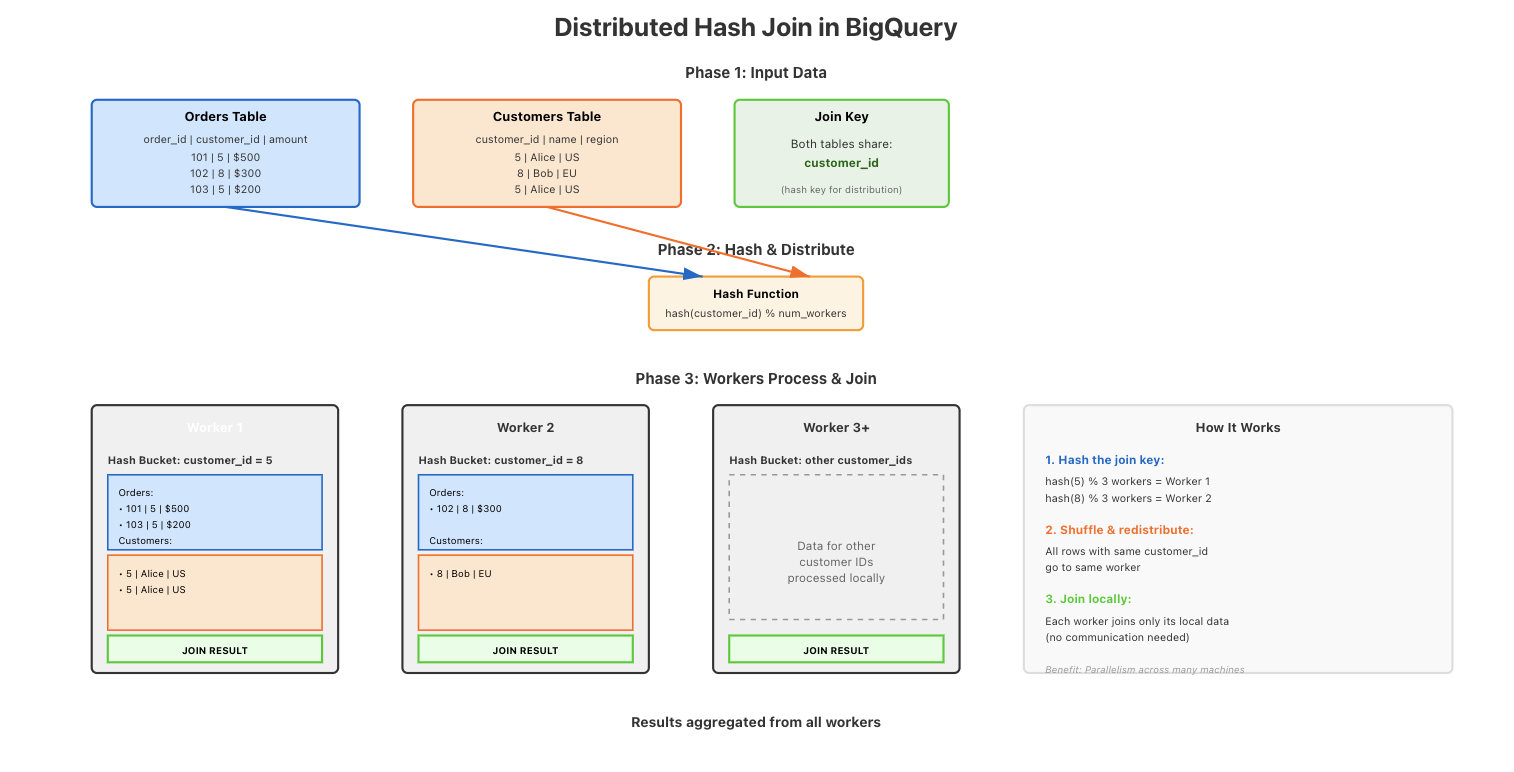
distributed hash joins
A distributed hash join means BigQuery splits the data across many machines.
Each machine:
- Hashes the join key (e.g., customer_id).
- Sends rows with the same hash to the same worker.
- Take the customer_id → run a hash function → result decides which worker gets the row.
- That worker joins only the matching rows it received.
Hashing ensures that matching rows from two tables go to the same machine, so the join can be done in parallel.
We hash the join key to keep the workload evenly distributed across all workers and avoid hotspots: highly imbalanced workload distributions.


Massively parallel
BigQuery is massively parallel because both the data and the query execution are distributed across many machines working at the same time.
- Data in BigQuery is stored in many chunks across distributed storage.
- When you run a query, BigQuery creates many workers (compute nodes).
- Each worker scans only its chunk of the data.
- All workers operate in parallel.
- Their partial results are then combined at the end.
So instead of one computer doing all the work, hundreds or thousands do small parts at once → massively parallel.
Partitioning
Columnar orientation splits the data with respect to columns. width / column reduction
BQ has a 2nd level of data reduction: partitionning : height / row reduction
Partitioning
Partitioning is splitting a large table into smaller chunks (partitions) based on a granular column — usually date, timestamp, or integer range.
Instead of scanning the whole table, BigQuery will only scan the partitions needed for the query.
- 2024-01-01 → partition
- 2024-01-02 → partition
- 2024-01-03 → partition
The query
SELECT * FROM events
WHERE event_date = "2024-01-02";
→ BigQuery reads only the 2024-01-02 partition, not the entire table.

Example
CREATE TABLE project.dataset.orders (
  order_id INT64,
  customer_id INT64,
  order_date DATE,
  amount FLOAT64
)
PARTITION BY DATE(order_date);
Or with extra clustering
CREATE TABLE project.dataset.customer_orders (
  order_id INT64,
  customer_id INT64,
  order_date DATE,
  region STRING,
  amount FLOAT64
)
PARTITION BY DATE(order_date)
CLUSTER BY customer_id, region;
Cluster by
CLUSTER BY further organizes the data within each partition into physical chunks.
Without clustering:
Partition: 2025-01-01
├── All rows for that date stored together
└── Mixed customer_ids and regions scattered throughout
With clustering:
Partition: 2025-01-01
├── Cluster 1: customer_id 1-100, region "US"
├── Cluster 2: customer_id 1-100, region "EU"
├── Cluster 3: customer_id 101-200, region "US"
└── Cluster 4: customer_id 101-200, region "EU"
The Physical Storage Benefit
When you query with a filter like:
SELECT * FROM customer_orders
WHERE DATE(order_date) = '2025-01-01'
  AND customer_id = 50
  AND region = 'US';
BigQuery does this:
- Partition pruning: Only reads the 2025-01-01 partition (skips all other dates)
- Cluster pruning: Within that partition, only reads Cluster 1 & 2 (skips clusters with customer_id > 100)
- Region pruning: Further narrows to just the “US” cluster
This dramatically reduces the amount of data read from disk—you’re scanning maybe 5-10% of the partition instead of 100%.
Key Point
Clustering creates sort order within the partition files. It doesn’t create separate sub-partitions you can see; it’s transparent internal organization.
But the physical data is ordered so that:
- Related rows (same customer_id, same region) are stored adjacently on disk
- BigQuery’s statistics know which file chunks contain which values
- Unnecessary file chunks can be skipped during queries
Recap
So partitioning is subseting a table wrt to rows while columnar data organization is subsetting a table wrt to columns.
- Columnar reduces width scanned.
- Partitioning + clustering reduces height scanned.
When you run a query:
SELECT col1, col3
FROM my_table
WHERE date = '2024-01-02';
BigQuery does this:
- Identify only the partition for
2024-01-02→ ignore all other row groups. - Inside that partition, read only col1 and col3 → ignore all other columns.
- Reassemble just those columns using row index alignment.
| Step | What is filtered | Effect |
|---|---|---|
| 1. Partition pruning | Rows | Skip irrelevant row blocks |
| 2. Column pruning | Columns | Skip irrelevant columns |
| 3. Join columns back | Based on row index | Reconstruct the requested rows |
Partitioning removes rows you don’t need, columnar storage skips columns you don’t need. -> BQ can handle super large datasets
but it’s not the only thing
1) Distributed Storage + Compute Separation
- Data lives in Colossus (Google’s distributed file system).
- Compute nodes don’t store data → they pull only what they need.
- Lets BigQuery scale compute independently of storage.
2) Massively Parallel Processing (MPP)
- A query is broken into many small tasks.
- Tasks run in parallel across many machines.
- More data → more workers → performance stays high.
3) Data Locality & Sharding
- Large tables are automatically sharded into chunks.
- Workers process chunks close to where they are stored, reducing network cost.
4) Compression + Encodings
Columns often contain similar values → BigQuery applies:
- Dictionary encoding
- Run-length encoding
- Delta encoding
Smaller data → lower scan cost → faster reads.
5) Broadcast + Distributed Hash Joins
Small tables are broadcast to all workers. : it is faster to copy the small table to every worker machine. Broadcasting means BigQuery copies the small table to all workers so each worker can join locally without moving large data around.
Large tables are joined in parallel using hash partitioning.
PostgreSQL performance is mainly about:
- Indexes → quickly find specific rows.
- Query planner / optimizer → choose best join + access strategy.
- Caching → keep hot data in RAM.
- Single-node execution → scale by using a bigger server.
Optimized for many small, precise lookups.
BigQuery performance is mainly about:
-
Subsetting the data before processing:
- Columnar storage → read only needed columns
- Partitioning → read only needed row ranges
- Further clustering → break partitions into parallel chunks
- Massively parallel execution across many workers
- Broadcast / distributed hash joins
- Vectorized execution + compression
Optimized for large scans and aggregations.
PostgreSQL goes fast by finding the right rows efficiently;
BigQuery goes fast by processing huge amounts of data in parallel while skipping everything it doesn’t need.
the user-facing SQL looks the same, but the execution model underneath is completely different.
You can write:
SELECT city, AVG(amount)
FROM orders
GROUP BY city;
This works in PostgreSQL and BigQuery.
But the engines behave differently
| Database | How it executes the SQL | What it’s optimized for |
|---|---|---|
| PostgreSQL | Uses indexes, row-level access, and a single-machine query planner | Fast small lookups and transactions |
| BigQuery | Skips columns, skips partitions, shards data, and runs work in parallel on many machines | Fast large scans and aggregations |