Postgresql Query performance - Explain - Scans
Query performance - Explain - Scans
The query planner
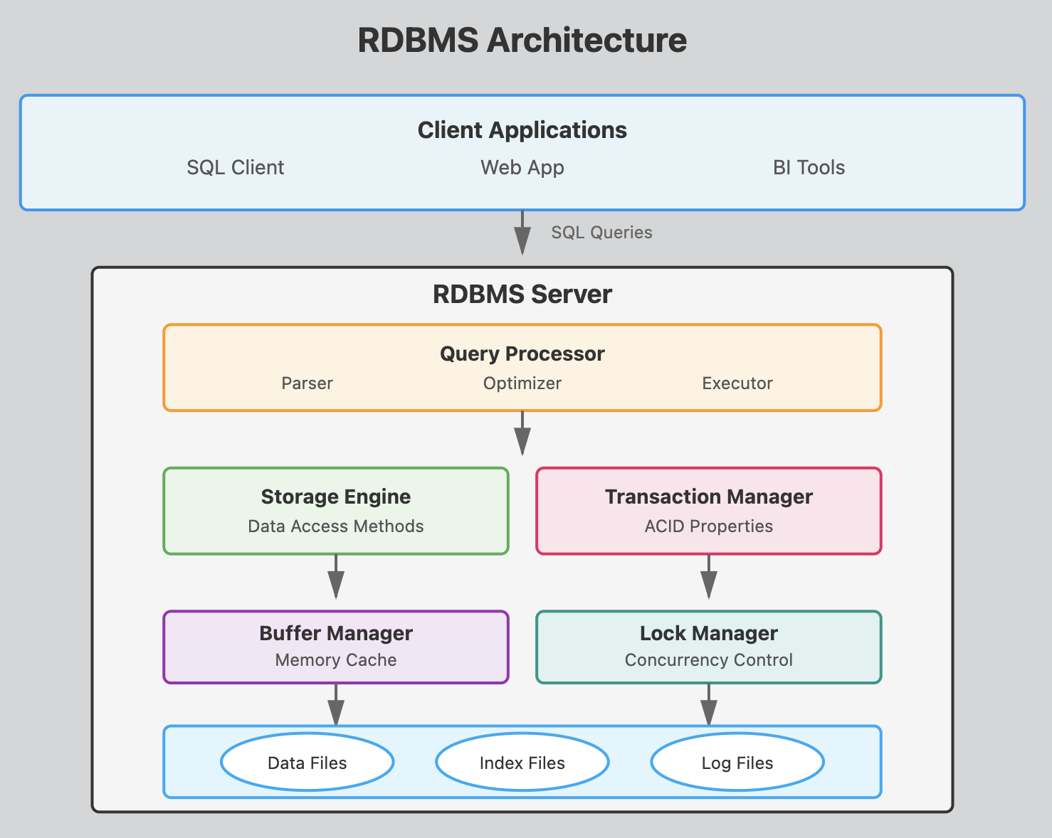
This architecture shows how a SQL query flows from the client through various processing layers before reaching the actual data on disk.
-
Parser: Checks SQL syntax and converts queries into an internal format the database can understand. It validates that tables and columns exist and that the user has proper permissions.
-
Optimizer: Determines the most efficient way to execute a query by analyzing different execution plans. It considers factors like available indexes, table statistics, and join methods to minimize resource usage. This is what makes
Postgresqlsuper efficient. -
Executor: Carries out the optimized query plan by coordinating with other components to retrieve or modify data according to the SQL command.
The database optimizer or query planner or engine chooses the most efficient method to deliver the results as expressed by the query.
The database optimizer interprets SQL queries along this process:
- compilation: transforms the query into a high level logical plan
- optimization: transforms logical plan into execution plan by choosing the most efficient algorithms for the job
- execution: executes the algorithms
Algorithms!
Here, think of algorithms as the actual physical operations that take place when the query plan is executed:
- getting to the data which is stored in memory or in physical storage,
- scanning the data,
- looking up indexes,
- filtering, sorting etc.
In the context of the PostgreSQL query optimizer, an algorithm is a systematic method to analyze, plan, and execute database queries efficiently.

Choosing the right Algorithm
How does the query planner chooses the best algorithms to execute the query ?
Many factors can be involved
- the nature of the tables and the data
- the query itself
- the type of filter (WHERE) operator
:=,<,between,like '%string'etc - the data types of the columns involved in the filters
- the number of rows of the table or the subqueries etc
- presence of
limit,order by, …
and
- the performance of the machine
(full text search is a topic by itself)
For each set of data (distribution, type) and table indexes, etc … there are specific rules and heuristics on which the query planner will base its choice of the most efficient algorithm to execute the query.
Understanding a query plan can be difficult.
Straight from the documentation : Plan-reading is an art that requires some experience to master, …. (🤣🤣🤣 emphasis here on the word art).
Planning and Cost reduction
Given a query, the role of the query planner is to find the most efficient way to execute it.
But what is efficient ?
Let’s say for the moment that efficient means fast.
The optimizer minimizes the cost of execution to lower execution time.:
- rewrites the query
- chooses the most efficient physical operations (i.e. algorithms) to execute the query
Cost function
However, the real execution time of a query also depends on the machine the server is running on. This machine may be brand new and powerful, or old and barely functionning. It may also be running processes that consume precious available resources.
The query optimizer does not have access to the overall machine context and the overall query time as experienced by the user is unknown to the optimizer. It also does not have access to external metrics such as monetary cost, user satisfaction, etc.
Instead the optimizer combines a measure of CPU cycles and I/O accesses to 1) derive a cost function and 2) minimize this cost function.
The query optimizer relies on resources that affect execution time: CPU cycles and I/O access which it combines into a single cost function that it tries to minimize.
Query costs
Depending on the machine that hosts the PostgresSQL server, PostgresSQL assigns different weights to these different variables to calculate the cost of a query
For instance, the cpu_operator_cost is defined as: Sets the planner’s estimate of the cost of processing each operator or function executed during a query. The default is 0.0025.
SHOW cpu_operator_cost;
returns:
 cpu_operator_cost
-------------------
 0.0025
Whereas, the cpu_tuple_cost is defined as : Sets the planner’s estimate of the cost of processing each row during a query. The default is 0.01.
There is a total of 13 cost related weights. Each dedicate to a specific operation. All have default values.
Blocks, storage and I/O access
There’s no magic. At the bottom of things, the database data is stored in files.
Let’s find where that data is with:
SHOW data_directory;
These are the folders you will find. The data is stored in base.
| Folder | Description |
|---|---|
base |
Stores actual data for user-created databases. |
global |
Contains system-wide metadata and cluster control files. |
pg_wal |
Write-Ahead Logs for transaction logging and recovery. |
pg_multixact |
Manages MultiXact transactions for row locking. |
pg_subtrans |
Tracks sub-transactions for nested transactions. |
pg_commit_ts |
Stores commit timestamps of transactions. |
pg_tblspc |
Symbolic links to tablespaces for external data storage. |
pg_stat_tmp |
Temporary statistics data for monitoring performance. |
pg_snapshots |
Stores transaction snapshots for MVCC isolation. |
pg_twophase |
Manages two-phase commit transactions. |
pg_logical |
Handles logical replication and WAL decoding. |
pg_replslot |
Stores replication slots for data streaming replication. |
pg_serial |
Tracks serializable transactions. |
pg_stat |
Collects statistics about database activity. |
pg_xact |
Tracks transaction commit/abort statuses. |
pg_dynshmem |
Stores dynamic shared memory for process coordination. |
take a minute to look it up on your machine
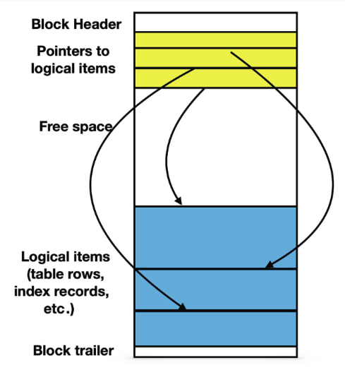
Blocks
Any file used for database objects is divided in blocks of the same length.
A block is the unit that is transfered between the hard drive and the main memory.
The number of I/O operations needed to execute any data access is equal to the number of blocks that are being read from or written to.
By default, PostgreSQL uses blocks containing 8192 bytes each.
Looking up one of the subfolders /1 of base:
ll  /usr/local/var/postgresql@16/base/1
total 15304
drwx------  301 alexis  admin   9.4K  6 Sep 09:05 .
drwx------   16 alexis  admin   512B 23 Sep 11:55 ..
-rw-------    1 alexis  admin   8.0K 22 Mar  2024 112
-rw-------    1 alexis  admin   8.0K 22 Mar  2024 113
-rw-------    1 alexis  admin   120K 22 Mar  2024 1247
-rw-------    1 alexis  admin    24K 22 Mar  2024 1247_fsm
-rw-------    1 alexis  admin   8.0K 22 Mar  2024 1247_vm
-rw-------    1 alexis  admin   456K 22 Mar  2024 1249
Several small items can reside in the same block; larger items may spread among several blocks.
EXPLAIN <SQL>
Postgresql optimization engine is excellent but sometimes needs troubleshooting.
The EXPLAIN <query> command outputs the execution plan of a query.
Important : The optimization engine will return different plans depending on the machine it runs on so the same query may result in different execution plans on different hardware.
Example
Let’s look at the query plan for a query on the movies database: the versatility_score query .
Just add EXPLAIN in front of the query:
EXPLAIN EXPLAIN WITH director_stats AS (
    SELECT
        d.name as director,
        COUNT(DISTINCT m.id) AS movie_count,
        COUNT(DISTINCT g.id) AS genre_count,
        ROUND(AVG(m.imdb_rating)::numeric, 2) AS avg_rating,
        ROUND(STDDEV(m.imdb_rating)::numeric, 2) AS rating_std
    FROM movies m
    JOIN directors d ON m.director_id = d.id
    LEFT JOIN movie_genres mg ON m.id = mg.movie_id
    LEFT JOIN genres g ON mg.genre_id = g.id
    WHERE m.imdb_rating IS NOT NULL
    GROUP BY d.name
    HAVING COUNT(DISTINCT m.id) >= 4
)
SELECT
    director,
    movie_count,
    genre_count,
    avg_rating,
    ROUND((genre_count::numeric * 2 + COALESCE(rating_std, 0)), 2) AS versatility_score
FROM director_stats;
The execution plan is:
QUERY PLAN
-------------
 Subquery Scan on director_stats  (cost=322.87..367.88 rows=183 width=94)
   ->  GroupAggregate  (cost=322.87..366.05 rows=183 width=94)
         Group Key: d.name
         Filter: (count(DISTINCT m.id) >= 4)
         ->  Sort  (cost=322.87..329.22 rows=2541 width=30)
               Sort Key: d.name, m.id
               ->  Hash Left Join  (cost=120.30..179.16 rows=2541 width=30)
                     Hash Cond: (mg.genre_id = g.id)
                     ->  Hash Join  (cost=118.83..169.67 rows=2541 width=30)
                           Hash Cond: (m.director_id = d.id)
                           ->  Hash Right Join  (cost=102.50..146.61 rows=2541 width=20)
                                 Hash Cond: (mg.movie_id = m.id)
                                 ->  Seq Scan on movie_genres mg  (cost=0.00..37.41 rows=2541 width=8)
                                 ->  Hash  (cost=90.00..90.00 rows=1000 width=16)
                                       ->  Seq Scan on movies m  (cost=0.00..90.00 rows=1000 width=16)
                                             Filter: (imdb_rating IS NOT NULL)
                           ->  Hash  (cost=9.48..9.48 rows=548 width=18)
                                 ->  Seq Scan on directors d  (cost=0.00..9.48 rows=548 width=18)
                     ->  Hash  (cost=1.21..1.21 rows=21 width=4)
                           ->  Seq Scan on genres g  (cost=0.00..1.21 rows=21 width=4)
(20 rows)
Lots of information!
Nodes
The output of EXPLAIN shows one node per line.
A node in a query plan represents a single operation or step in the execution of a query.
Each node describes a specific action that Postgres will execute, such as
- scanning a table,
- applying a filter,
- joining tables,
- or sorting results.
and information such as an estimation of the associated cost, the number of rows etc …
Nodes are arranged in a tree structure, with child nodes feeding results to their parent nodes, ultimately leading to the final result of the query.
Sequential Scan
Let’s look at the query plan for a simple select query. (on the treesdb_v03_normalized database)
explain select * from trees;
                          QUERY PLAN
--------------------------------------------------------------
 Seq Scan on trees  (cost=0.00..4869.39 rows=211339 width=49)
(1 row)
The operation is a Sequential Scan on the trees table.
Sequential Scan: the algorithm is simply reading all rows from the table in order, from beginning to end. It’s the most straightforward way to retrieve all data when no filtering is required.
The query plan shows:
- The estimated cost ranges from 0.00 (start-up cost) to 4577.39 (total cost).
- It expects to return 211,339 rows. (which is in fact the number of rows on the
treestable) - The average width of each row is estimated to be 49 bytes.
Note: The width is the estimated average size of each returned row in bytes.
Since we’re selecting all columns and all rows, PostgreSQL has no choice but to read the entire table sequentially.
A Sequential Scan is the most efficient method for retrieving all data from a table.
The Cost of a Sequential Scan
The estimated cost for a Sequential Scan is computed as :
(number of pages read from disk * seq_page_cost) + (rows scanned * cpu_tuple_cost).
By default, seq_page_cost = 1.0 and cpu_tuple_cost = 0.01,
see https://www.postgresql.org/docs/current/runtime-config-query.html#GUC-SEQ-PAGE-COST and https://www.postgresql.org/docs/current/runtime-config-query.html#GUC-CPU-TUPLE-COST
We can lookup the number of pages for a given table with
SELECT relname, relkind, reltuples, relpages
FROM pg_class
WHERE relname = 'trees';
which returns
  relname    | relkind | reltuples | relpages
--------------+---------+-----------+----------
 trees        | r       |    211339 |     2756
The trees table occupies 2756 pages and has 211339 tuples (rows).
So the estimated cost is (2756 * 1.0) + (211339 * 0.01) = 4869.39 which is the exact number shown in the query plan.
The pg_class table
The pg_class table in PostgreSQL is a system catalog that contains metadata about tables, indexes, sequences, views, and other relation-like objects.
| Column | Description |
|---|---|
relname |
Name of the relation (table, index, etc.). |
reltuples |
Estimated number of rows in the table or index. |
relpages |
Number of disk pages that the table or index uses (approximate). |
relkind |
Type of relation: ‘r’ (table), ‘i’ (index), ‘S’ (sequence), ‘v’ (view), etc. |
relhasindex |
true if the table has any indexes. |
... |
other columns |
pg_class tracks:
- Tables and Views
- Indexes
- Sequences
- Materialized Views
- Partitions
EXPLAIN ANALYZE
EXPLAIN ANALYZE complements the EXPLAIN command by also sampling the data and calculating statistics that will be used to optimize the plan.
While EXPLAIN uses default statistical estimates about the data, EXPLAIN ANALYZE uses real stats.
Furthermore, EXPLAIN ANALYZE
- effectively runs the query (but does not display the output)
And returns:
- the real execution time
- the true number of rows
It also outputs:
- I/O timings: time spent on I/O operations.
- Worker information: Details about workers used in parallel queries.
- Memory usage: memory used during query execution.
- Buffers information: details about shared and local buffer usage, including hits and reads.
for instance :
EXPLAIN ANALYZE select * from trees where height < 9;
returns
                                                  QUERY PLAN
---------------------------------------------------------------------------------------------------------------
 Seq Scan on trees  (cost=0.00..5397.74 rows=111066 width=49) (actual time=0.661..144.453 rows=111594 loops=1)
   Filter: (height < 9)
   Rows Removed by Filter: 99745
 Planning Time: 0.068 ms
 Execution Time: 152.224 ms
EXPLAIN ANALYZE on updates
Since EXPLAIN ANALYZE actually runs the query, you have to be cautious when using it on UPDATE, INSERT or DELETE queries 🧨🧨🧨
The best pratice is to use EXPLAIN first to get a rough idea about possible optimizations then after you’ve optimized the tables and your query, and then run EXPLAIN ANALYZE to get an accurate timing of the query execution
Rollback
To analyze a data-modifying query without changing the tables, wrap the EXPLAIN ANALYZE statement between BEGIN and ROLLBACK. That way the query will be rolled back after its execution.
For instance:
BEGIN;

EXPLAIN ANALYZE UPDATE trees SET height = height / 10 WHERE height > 100;

ROLLBACK;
EXPLAIN : WHERE clause
Let’s add a where clause on the height attribute, to our simple select * from trees; and see what the optimizer makes of it
EXPLAIN select * from trees where height < 9;
returns:
                          QUERY PLAN
--------------------------------------------------------------
 Seq Scan on trees  (cost=0.00..5397.74 rows=111066 width=49)
   Filter: (height < 9)
(2 rows)
Compare that to the original query plan without the filter:
                          QUERY PLAN
--------------------------------------------------------------
 Seq Scan on trees  (cost=0.00..4869.39 rows=211339 width=50)
So the cost has gone up (4869.39 -> 5397.74) while the number of rows has gone down (211339 -> 111270) !
We’re asking the Seq Scan node to check the condition for each row it scans, and outputs only the ones that pass the condition.
The estimate of output rows has been reduced because of the WHERE clause.
However, the scan still has to visit all 211339 rows, so the cost hasn’t decreased; in fact it has gone up a bit (by 211339 * cpu_operator_cost you can check) to reflect the extra CPU time spent checking the WHERE condition.
treesdb_v04=# SHOW cpu_operator_cost;
 cpu_operator_cost
-------------------
 0.0025
(1 row)
Now the cost is given by
(number of pages read from disk * seq_page_cost) + \
(rows scanned * cpu_tuple_cost) + \
(rows scanned * cpu_operator_cost)
The impact of indexing and Bitmap Scans
The trees table has a primary key id shown by the index
\d+ trees
Indexes:
    "trees_pkey" PRIMARY KEY, btree (id)
Access method: heap
Let’s see how this index trees_pkey is put to use by the query planner when we filter on id instead of height
EXPLAIN select * from trees where id < 1000
We get
                                  QUERY PLAN
------------------------------------------------------------------------------
 Bitmap Heap Scan on trees  (cost=32.28..2039.27 rows=1014 width=49)
   Recheck Cond: (id < 1000)
   ->  Bitmap Index Scan on trees_pkey  (cost=0.00..32.03 rows=1014 width=0)
         Index Cond: (id < 1000)
 (4 rows)
The query planner executed a two step plan where the child node: Bitmap Index Scan feeds the rows into a parent node: Bitmap Heap Scan.
HEAP meaning the entire block.
The overall costs has gone down since the parent scan only has to check the filtering condition on 10k rows.
Notice that the number of rows is not correct: 1014 instead of 999. EXPLAIN gives out estimates not exact numbers.
BITMAP
A bitmap is a compact data structure used to represent a set of row identifiers.
- Structure: It is essentially an array of bits (0s and 1s).
- Representation: Each bit corresponds to a row in the table. A ‘1’ indicates the row matches the query condition, while a ‘0’ means it doesn’t.
- Efficiency: Bitmaps are memory-efficient for representing large sets of rows, especially when dealing with millions of records.
- Operations: Bitmaps allow for quick set operations (AND, OR, NOT) when combining multiple conditions.
- Purpose: In a Bitmap Heap Scan, the bitmap helps the database quickly identify which rows need to be fetched from the table, avoiding unnecessary I/O.

Difference between Bitmap Heap Scan and Sequential Scan
-
Sequential Scan :
- Reads all rows in the table sequentially, one after another.
- Doesn’t use any index.
- Efficient for reading a large portion of the table.
-
Bitmap Heap Scan: Uses a two-step process:
- a) First, it creates a bitmap in memory where each bit represents a table block.
- b) Then, it actually fetches the rows from the table based on this bitmap.
- Often used when an index scan returns a moderate number of rows.
The key difference lies in how these methods access the data:
-
Reading sequentially in Sequential Scan: The database reads all data pages in order, one after another. This is efficient because it follows the natural order of data on disk.
-
Fetching rows separately in Bitmap Heap Scan: After creating the bitmap, the database jumps around the table to fetch only the specific rows that match the condition.
This involves more random I/O operations, which are generally slower than sequential reads.
In the end, the cost is lower with a bitmap scan because the planner has to deal with a much smaller number of rows
BUT: if the filtering is less stringent, the planner will revert back to a Sequential Scan
For instance:
treesdb_v04=# EXPLAIN select * from trees where id < 150000;
                          QUERY PLAN
--------------------------------------------------------------
 Seq Scan on trees  (cost=0.00..5105.74 rows=149967 width=50)
   Filter: (id < 150000)
(2 rows)
Because in that case since the filtering is too large, the advantage of using a bitmap scan becomes too small.
Note: We could probably plot a curve by increasing the id threshold and seeing when the cutoff from Sequential Scan to Bitmap Scan occurs
Index Scan
If the column is part of an index, then the planner can decide to directly use the index with an Index Scan
Index Scans are used for:
-
High Selectivity Queries: when the query is expected to return a small portion of the table’s rows, typically less than 5-10%. The index allows quick access to these few rows without scanning the entire table.
-
Ordered Results: when the query requires results in the order of the index (e.g., ORDER BY clause matches the index order). The index already maintains data in sorted order, avoiding a separate sorting step.
-
Unique Constraints: for queries looking up rows based on a unique or primary key. These are typically very fast as they return at most one row.
Index Scan Example
treesdb_v04=# explain select * from trees where id = 808;
                               QUERY PLAN
-------------------------------------------------------------------------
 Index Scan using trees_pkey on trees  (cost=0.42..8.44 rows=1 width=50)
   Index Cond: (id = 808)
3 types of scans
We already have threes types of scans:
- Sequential Scan
- Bitmap Scan
- Index Scan
Let’s recap
the Index Scan
- Used when: Fetching a small number of rows based on an index condition.
- How it works:
- Directly uses the index to find the location of rows matching the condition.
- Then fetches those specific rows from the table.
- Efficiency: Very efficient for retrieving a small number of rows, especially with highly selective conditions.
- In your example: It’s using the primary key index (trees_pkey) to quickly find the row with id = 808.
the Bitmap Heap Scan
-
Used when: Fetching a moderate number of rows based on an index condition.
- How it works:
- Two-step process: a) First, creates a bitmap in memory where each bit represents a table block that contains matching rows. b) Then, fetches the actual rows from the table based on this bitmap.
- Efficiency: More efficient than Index Scan when retrieving a larger number of rows, but still selective enough not to warrant a full Sequential Scan.
the Sequential Scan
-
Used when: Reading a large portion of the table or when no suitable index is available.
- How it works:
- Reads all rows in the table sequentially, one after another.
- Checks each row against the condition (if any).
- Efficiency: Efficient for reading large portions of a table, but can be slow for selective queries on large tables.
The Key differences are:
- Data access pattern:
- Index Scan: Might jump around the table to fetch specific rows.
- Sequential Scan: Reads the entire table sequentially.
- Bitmap Heap Scan: First creates a map of relevant blocks, then fetches those blocks (which can be more organized than Index Scan but less sequential than Sequential Scan).
- Use of indexes:
- Index Scan: Directly uses the index.
- Sequential Scan: Doesn’t use any index.
- Bitmap Heap Scan: Uses an index to create the bitmap, then accesses the table.
- Suitability for different data volumes:
- Index Scan: Best for very selective queries (few rows).
- Seq Scan: Best for reading large portions of the table.
- Bitmap Heap Scan: Good middle ground for moderate selectivity.
Key Takeaways
Query Optimization
- The query planner chooses HOW to execute your query - You write WHAT you want (declarative SQL), PostgreSQL figures out the fastest way to get it
- Cost function drives decisions - PostgreSQL estimates costs using CPU cycles and I/O operations, then picks the cheapest execution plan
- Same query, different plans - The optimizer may choose different strategies depending on your hardware, data distribution, and available indexes
Physical Operations (Algorithms)
- Sequential Scan - Reads all rows from start to finish; best when retrieving most of the table
- Index Scan - Uses an index to jump directly to specific rows; fastest for highly selective queries (finding 1 or a few rows)
- Bitmap Heap Scan - Middle ground that combines index lookup with organized data fetching; good for moderate selectivity
Data Storage
- Data lives in blocks - PostgreSQL stores data in 8KB blocks on disk
- I/O is expensive - Reading blocks from disk is slow, so minimizing block reads is crucial for performance
- Indexes reduce I/O - They help skip irrelevant data instead of scanning everything
Using EXPLAIN
- EXPLAIN shows the plan - See what PostgreSQL will do before running the query
- EXPLAIN ANALYZE shows reality - Actually runs the query and reports real timing and row counts
- Cost estimates aren’t guarantees - EXPLAIN uses statistics; EXPLAIN ANALYZE uses real data
- Watch out with ANALYZE on updates - It actually executes the query, so wrap in BEGIN/ROLLBACK for safety
Practical Wisdom
- Indexes don’t always help - For large result sets, sequential scans are faster than using indexes
- Filter selectivity matters - The more selective your WHERE clause (fewer rows), the more likely indexes help
- Reading query plans is an art - Takes practice to understand what the optimizer is doing and why