Window Functions CTEs Lab

window functions, CTEs, trees database, data quality

dataset

We’ll work on the normalized version of the trees db

download the sql backup from https://skatai.com/assets/db/treesdb_v03_normalized.sql
restore the database

from the terminal

psql -d postgres -f <path to the sql backup>/treesdb_v03_normalized.sql

or within a PSQL session

\i <path to the sql backup>/treesdb_v03_normalized.sql

This will create a new database called treesdb_v03_normalized

Explore

Check out the tables, make a few queries to get a sense of the data.

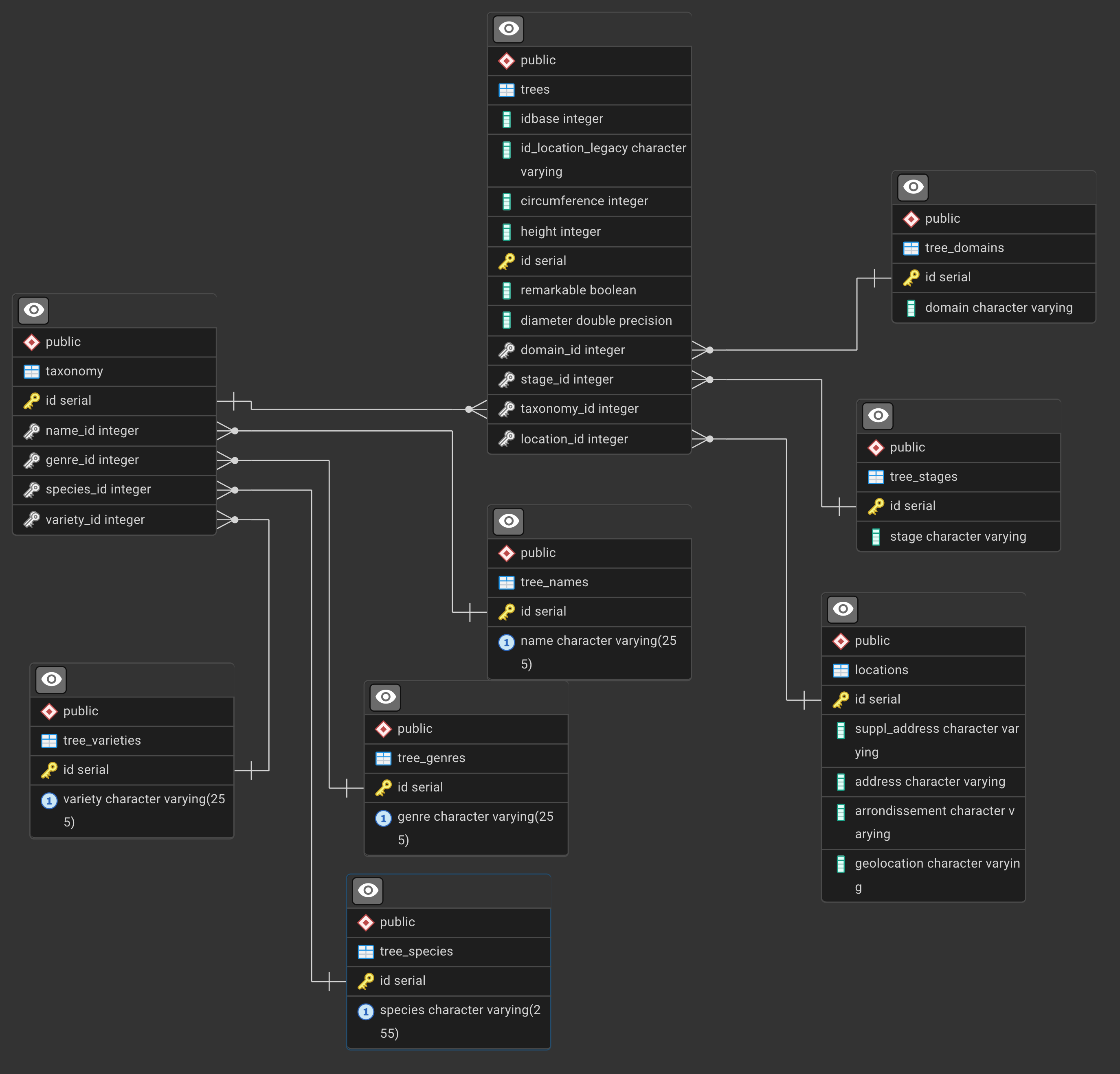
The ERD is

moviesdb

PostgreSQL Window Functions Exercises: Paris Trees Database

This comprehensive series of exercises will help you master window functions in PostgreSQL using a real-world dataset of trees in Paris.

important: all results are obtained after ordering by random() and limiting to a few rows. all your queries should also be ordered by random() and limited to a few rows.

Exercise 1: Basic Window Functions - Tree Count by Arrondissement

Goal: For each tree, show its arrondissement and the total count of trees in that arrondissement.

Concepts: Basic COUNT() window function with OVER(PARTITION BY)

Step-by-step guide:

Start with the main trees table
Join with locations to get arrondissement information
Use COUNT(*) OVER (PARTITION BY arrondissement) to count trees per arrondissement
Select the tree id, arrondissement, and the count

Hints:

Window functions don’t reduce rows like GROUP BY does
Each tree row will show the total count for its arrondissement
The PARTITION BY clause divides the data into groups for the window function

For comparison - GROUP BY approach:

results

   id   |  arrondissement   | trees_in_arrondissement
--------+-------------------+-------------------------
 108631 | PARIS 16E ARRDT   |                   17128
 208989 | PARIS 1ER ARRDT   |                    1645
  18713 | PARIS 13E ARRDT   |                   17462
 159547 | PARIS 19E ARRDT   |                   15235

Solution:

SELECT
    t.id,
    l.arrondissement,
    COUNT(*) OVER (PARTITION BY l.arrondissement) as trees_in_arrondissement
FROM trees t
JOIN locations l ON t.location_id = l.id
WHERE l.arrondissement IS NOT NULL
ORDER BY trees_in_arrondissement DESC, l.arrondissement;

SELECT
    l.arrondissement,
    COUNT(*) as tree_count
FROM trees t
JOIN locations l ON t.location_id = l.id
WHERE l.arrondissement IS NOT NULL
GROUP BY l.arrondissement
ORDER BY tree_count DESC;

Exercise 2: Finding the Tallest Tree per Arrondissement

Goal: For each tree, show how its height compares to the maximum height in its arrondissement.

Concepts: MAX() window function, comparing values to aggregates

Step-by-step guide:

Join trees and locations tables
Use MAX(height) OVER (PARTITION BY arrondissement) to find the tallest tree per area
Calculate the difference between each tree’s height and the maximum
Filter to only show trees with valid heights

Hints:

You can use multiple columns in your SELECT with window functions
Consider what height - MAX(height) OVER (...) tells you
Trees with a difference of 0 are the tallest in their arrondissement

to get a better view of the results, you can limit the number of rows returned and order by random()

ORDER BY random() <other order by> limit 20;

Solution:

SELECT
    t.id,
    l.arrondissement,
    t.height,
    MAX(t.height) OVER (PARTITION BY l.arrondissement) as max_height_in_area,
    t.height - MAX(t.height) OVER (PARTITION BY l.arrondissement) as diff_from_max
FROM trees t
JOIN locations l ON t.location_id = l.id
WHERE t.height IS NOT NULL
    AND l.arrondissement IS NOT NULL
ORDER BY random() , l.arrondissement, diff_from_max DESC limit 20;

results

   id   |  arrondissement   | height | max_height_in_area | diff_from_max
--------+-------------------+--------+--------------------+---------------
   5422 | PARIS 11E ARRDT   |     35 |                 35 |             0
 133998 | PARIS 20E ARRDT   |     15 |                 30 |           -15
  61004 | BOIS DE VINCENNES |     10 |                120 |          -110
  86518 | PARIS 20E ARRDT   |     12 |                 30 |           -18

Exercise 3: Data Quality - Missing Heights by Genre

Here’s the corrected query for Exercise 3:

Exercise 3: Data Quality - Missing Heights by Genre

Goal: Identify genres with missing height data by showing the count and percentage of trees with missing (0) heights.

Concepts: COUNT() with conditions, calculating percentages with window functions

Step-by-step guide:

Join trees with taxonomy and tree_genres tables
Use COUNT(*) OVER (PARTITION BY genre) for total trees per genre
Use COUNT(CASE WHEN height > 0 THEN 1 END) OVER (PARTITION BY genre) for trees with valid heights
Calculate the difference to find missing values (height = 0)
Compute percentage of missing data

Hints:

In this dataset, missing heights are stored as 0, not NULL
COUNT(CASE WHEN height > 0 THEN 1 END) only counts trees with actual height values
COUNT(*) counts all rows
The difference gives you the count of missing/zero heights
Use DISTINCT in the outer query to avoid repeated calculations

Solution:

SELECT DISTINCT
    tg.genre,
    COUNT(*) OVER (PARTITION BY tg.genre) as total_trees,
    COUNT(CASE WHEN t.height > 0 THEN 1 END) OVER (PARTITION BY tg.genre) as trees_with_height,
    COUNT(CASE WHEN t.height = 0 THEN 1 END) OVER (PARTITION BY tg.genre) as missing_height,
    ROUND(100.0 * COUNT(CASE WHEN t.height = 0 THEN 1 END) OVER (PARTITION BY tg.genre) /
          COUNT(*) OVER (PARTITION BY tg.genre), 2) as pct_missing
FROM trees t
JOIN taxonomy tx ON t.taxonomy_id = tx.id
JOIN tree_genres tg ON tx.genre_id = tg.id
ORDER BY pct_missing DESC;

Alternative approach (more explicit):

SELECT DISTINCT
    tg.genre,
    COUNT(*) OVER (PARTITION BY tg.genre) as total_trees,
    COUNT(*) OVER (PARTITION BY tg.genre) - COUNT(CASE WHEN t.height = 0 THEN 1 END) OVER (PARTITION BY tg.genre) as trees_with_height,
    COUNT(CASE WHEN t.height = 0 THEN 1 END) OVER (PARTITION BY tg.genre) as missing_height,
    ROUND(100.0 * COUNT(CASE WHEN t.height = 0 THEN 1 END) OVER (PARTITION BY tg.genre) /
          COUNT(*) OVER (PARTITION BY tg.genre), 2) as pct_missing
FROM trees t
JOIN taxonomy tx ON t.taxonomy_id = tx.id
JOIN tree_genres tg ON tx.genre_id = tg.id
ORDER BY pct_missing DESC;

results

       genre       | total_trees | trees_with_height | missing_height | pct_missing
-------------------+-------------+-------------------+----------------+-------------
 Rhododendron      |           8 |                 0 |              8 |      100.00
 Podocarpus        |           2 |                 0 |              2 |      100.00
 Tsuga             |           1 |                 0 |              1 |      100.00
 Cephalotaxus      |           1 |                 0 |              1 |      100.00
 Juniperus         |           5 |                 0 |              5 |      100.00
 Cercidiphyllum    |           8 |                 1 |              7 |       87.50

Note: a SQL query with GROUP BY would be simpler,

For instance

SELECT
    tg.genre,
    COUNT(*) as total_trees,
    COUNT(CASE WHEN t.height > 0 THEN 1 END) as trees_with_height,
    COUNT(CASE WHEN t.height = 0 THEN 1 END) as missing_height,
    ROUND(100.0 * COUNT(CASE WHEN t.height = 0 THEN 1 END) / COUNT(*), 2) as pct_missing
FROM trees t
JOIN taxonomy tx ON t.taxonomy_id = tx.id
JOIN tree_genres tg ON tx.genre_id = tg.id
GROUP BY tg.genre
ORDER BY pct_missing DESC;

Exercise 4: ROW_NUMBER - Ranking Trees by Height within Each Domain

Goal: Assign a sequential ranking to trees by height within each domain.

Concepts: ROW_NUMBER(), ordering within partitions

Step-by-step guide:

Join trees with tree_domains
Use ROW_NUMBER() OVER (PARTITION BY domain ORDER BY height DESC)
Filter for trees that have height values
Show only the top 5 trees per domain

Hints:

ROW_NUMBER() always gives unique sequential numbers (1, 2, 3, …)
Use a subquery to filter by row_number (you can’t use window functions in WHERE directly)
ORDER BY height DESC puts tallest trees first

Query Skeleton:

SELECT * FROM (
    SELECT
        ...,
        ROW_NUMBER() OVER (...) as rn
    FROM ...
    WHERE ...
) subquery
WHERE rn <= 5;

Solution:

SELECT * FROM (
    SELECT
        t.id,
        td.domain,
        t.height,
        ROW_NUMBER() OVER (PARTITION BY td.domain ORDER BY t.height DESC) as height_rank
    FROM trees t
    JOIN tree_domains td ON t.domain_id = td.id
    WHERE t.height IS NOT NULL
        AND td.domain IS NOT NULL
) ranked
WHERE height_rank <= 5
ORDER BY domain, height_rank;

results

   id   |    domain    | height | height_rank
--------+--------------+--------+-------------
 172122 | Alignement   |   2524 |           1
 152402 | Alignement   |   2019 |           2
 166842 | Alignement   |    720 |           3
 168045 | Alignement   |    225 |           4
  93247 | Alignement   |    200 |           5
  88686 | CIMETIERE    |    119 |           1
  91418 | CIMETIERE    |    116 |           2
  91576 | CIMETIERE    |     35 |           3

Exercise 5: RANK vs DENSE_RANK - Handling Ties in Circumference

Goal: Compare RANK() and DENSE_RANK() behavior when trees have the same circumference within each arrondissement.

Concepts: RANK(), DENSE_RANK(), understanding ties

Step-by-step guide:

Join trees with locations
Apply both RANK() and DENSE_RANK() with the same ordering
Order by circumference descending within each arrondissement
Show the difference between the two ranking methods

Hints:

RANK() leaves gaps after ties: 1, 2, 2, 4, 5
DENSE_RANK() has no gaps: 1, 2, 2, 3, 4
Look for trees with the same circumference to see the difference
Limit results to make patterns visible

Solution:

SELECT
    t.id,
    l.arrondissement,
    t.circumference,
    RANK() OVER (PARTITION BY l.arrondissement ORDER BY t.circumference DESC) as rank_with_gaps,
    DENSE_RANK() OVER (PARTITION BY l.arrondissement ORDER BY t.circumference DESC) as dense_rank_no_gaps,
    RANK() OVER (PARTITION BY l.arrondissement ORDER BY t.circumference DESC) -
        DENSE_RANK() OVER (PARTITION BY l.arrondissement ORDER BY t.circumference DESC) as gap_size
FROM trees t
JOIN locations l ON t.location_id = l.id
WHERE t.circumference IS NOT NULL
    AND l.arrondissement IS NOT NULL
ORDER BY l.arrondissement, t.circumference DESC
LIMIT 100;

Exercise 6: Detecting Outliers - Heights Beyond 2 Standard Deviations

Goal: Identify unusually tall or short trees by comparing them to statistical measures within their species.

Concepts: AVG(), STDDEV() window functions, statistical outlier detection

Step-by-step guide:

Join trees, taxonomy, and tree_species tables
Calculate AVG(height) and STDDEV(height) per species using window functions
Compute z-score: (height - avg) / stddev
Filter for trees where absolute z-score > 2
Use a subquery since you need to filter on calculated window function results

Hints:

A z-score shows how many standard deviations a value is from the mean
Z-score > 2 or < -2 typically indicates an outlier
ABS() function gets absolute value
Only include species with enough trees for meaningful statistics

Query Skeleton:

SELECT * FROM (
    SELECT
        ...,
        AVG(...) OVER (PARTITION BY ...) as avg_height,
        STDDEV(...) OVER (PARTITION BY ...) as stddev_height,
        (height - AVG(...) OVER (...)) / STDDEV(...) OVER (...) as z_score
    FROM ...
    WHERE ...
) stats
WHERE ABS(z_score) > 2
    AND stddev_height IS NOT NULL;

Solution:

SELECT * FROM (
    SELECT
        t.id,
        ts.species,
        t.height,
        AVG(t.height) OVER (PARTITION BY ts.species) as avg_species_height,
        STDDEV(t.height) OVER (PARTITION BY ts.species) as stddev_species_height,
        COUNT(*) OVER (PARTITION BY ts.species) as species_count,
        (t.height - AVG(t.height) OVER (PARTITION BY ts.species)) /
            NULLIF(STDDEV(t.height) OVER (PARTITION BY ts.species), 0) as z_score
    FROM trees t
    JOIN taxonomy tx ON t.taxonomy_id = tx.id
    JOIN tree_species ts ON tx.species_id = ts.id
    WHERE t.height IS NOT NULL
) outlier_analysis
WHERE ABS(z_score) > 2
    AND stddev_species_height IS NOT NULL
    AND species_count >= 30
ORDER BY ABS(z_score) DESC;

Exercise 7: Distribution Analysis - Percentile Ranks for Tree Diameter

Goal: Calculate what percentage of trees in each domain have a smaller diameter than each tree.

Concepts: PERCENT_RANK(), CUME_DIST(), understanding percentiles

Step-by-step guide:

Join trees with tree_domains
Use PERCENT_RANK() to get relative rank (0 to 1)
Use CUME_DIST() to get cumulative distribution
Convert to percentages for easier interpretation
Filter for valid diameter and domain values

Hints:

PERCENT_RANK() returns 0 for the smallest value, 1 for the largest
CUME_DIST() returns the fraction of rows <= current row
Multiply by 100 to convert to percentages
These help you understand distribution within groups

Solution:

SELECT
    t.id,
    td.domain,
    t.diameter,
    PERCENT_RANK() OVER (PARTITION BY td.domain ORDER BY t.diameter) as pct_rank,
    ROUND(100 * PERCENT_RANK() OVER (PARTITION BY td.domain ORDER BY t.diameter), 2) as percentile,
    CUME_DIST() OVER (PARTITION BY td.domain ORDER BY t.diameter) as cum_dist,
    ROUND(100 * CUME_DIST() OVER (PARTITION BY td.domain ORDER BY t.diameter), 2) as pct_at_or_below
FROM trees t
JOIN tree_domains td ON t.domain_id = td.id
WHERE t.diameter IS NOT NULL
    AND td.domain IS NOT NULL
ORDER BY td.domain, t.diameter DESC
LIMIT 200;

Exercise 8: Multi-Level Ranking - Best Trees by Species within Each Arrondissement

Goal: Create a two-level ranking showing the tallest trees of each species within each arrondissement.

Concepts: Multiple window functions, complex partitioning

Step-by-step guide:

Join trees, locations, taxonomy, and tree_species
Create a ranking by height within each (arrondissement, species) combination
Also show how this tree ranks across all species in that arrondissement
Filter to show only top 3 per species per arrondissement
Use subquery to filter on window function results

Hints:

You can have multiple OVER() clauses with different PARTITION BY conditions
First partition: PARTITION BY arrondissement, species
Second partition: PARTITION BY arrondissement
This shows both local (within species) and global (within area) rankings

Query Skeleton:

SELECT * FROM (
    SELECT
        ...,
        ROW_NUMBER() OVER (PARTITION BY arr, species ORDER BY height DESC) as rank_in_species,
        ROW_NUMBER() OVER (PARTITION BY arr ORDER BY height DESC) as rank_in_area
    FROM ...
    JOIN ... ON ...
    WHERE ...
) ranked
WHERE rank_in_species <= 3;

Solution:

SELECT * FROM (
    SELECT
        t.id,
        l.arrondissement,
        ts.species,
        t.height,
        ROW_NUMBER() OVER (PARTITION BY l.arrondissement, ts.species
                          ORDER BY t.height DESC) as rank_within_species,
        ROW_NUMBER() OVER (PARTITION BY l.arrondissement
                          ORDER BY t.height DESC) as rank_in_arrondissement,
        COUNT(*) OVER (PARTITION BY l.arrondissement, ts.species) as species_count_in_area
    FROM trees t
    JOIN locations l ON t.location_id = l.id
    JOIN taxonomy tx ON t.taxonomy_id = tx.id
    JOIN tree_species ts ON tx.species_id = ts.id
    WHERE t.height IS NOT NULL
        AND l.arrondissement IS NOT NULL
        AND ts.species IS NOT NULL
) ranked_trees
WHERE rank_within_species <= 3
    AND species_count_in_area >= 10
ORDER BY arrondissement, species, rank_within_species;

Exercise 9: Data Quality - Identifying Imbalanced Remarkable Trees

Goal: Analyze the distribution of the remarkable flag, showing how imbalanced it is across different domains and stages.

Concepts: Conditional aggregation with window functions, handling boolean/NULL values

Step-by-step guide:

Join trees with tree_domains and tree_stages
Count total trees per domain/stage combination
Count trees where remarkable = true
Count trees where remarkable IS NULL
Calculate percentages for each category
Use DISTINCT to avoid row repetition

Hints:

COUNT(CASE WHEN remarkable = true THEN 1 END) counts only TRUE values
COUNT(CASE WHEN remarkable IS NULL THEN 1 END) counts NULLs
Window functions with CASE statements are powerful for conditional counting
This reveals data quality issues with the remarkable flag

Query Skeleton:

SELECT DISTINCT
    domain,
    stage,
    COUNT(*) OVER (PARTITION BY ...) as total,
    COUNT(CASE WHEN ... THEN 1 END) OVER (PARTITION BY ...) as remarkable_count,
    COUNT(CASE WHEN ... IS NULL THEN 1 END) OVER (PARTITION BY ...) as null_count,
    -- percentages
FROM ...
ORDER BY ...;

Solution:

SELECT DISTINCT
    td.domain,
    ts.stage,
    COUNT(*) OVER (PARTITION BY td.domain, ts.stage) as total_trees,
    COUNT(CASE WHEN t.remarkable = true THEN 1 END) OVER (PARTITION BY td.domain, ts.stage) as remarkable_count,
    COUNT(CASE WHEN t.remarkable IS NULL THEN 1 END) OVER (PARTITION BY td.domain, ts.stage) as null_count,
    ROUND(100.0 * COUNT(CASE WHEN t.remarkable = true THEN 1 END) OVER (PARTITION BY td.domain, ts.stage) /
          COUNT(*) OVER (PARTITION BY td.domain, ts.stage), 2) as pct_remarkable,
    ROUND(100.0 * COUNT(CASE WHEN t.remarkable IS NULL THEN 1 END) OVER (PARTITION BY td.domain, ts.stage) /
          COUNT(*) OVER (PARTITION BY td.domain, ts.stage), 2) as pct_null
FROM trees t
LEFT JOIN tree_domains td ON t.domain_id = td.id
LEFT JOIN tree_stages ts ON t.stage_id = ts.id
ORDER BY total_trees DESC;

Exercise 10: Running Totals - Cumulative Tree Count by Circumference Range

Goal: Create a running total showing how many trees exist at or below each circumference threshold within each genus.

Concepts: SUM() with window frames, running totals, ROWS BETWEEN

Step-by-step guide:

Join trees, taxonomy, and tree_genres
Order trees by circumference within each genus
Use SUM(1) OVER (PARTITION BY genus ORDER BY circumference ROWS BETWEEN UNBOUNDED PRECEDING AND CURRENT ROW)
This creates a running count
Round circumferences to groups (e.g., multiples of 10) for clearer analysis

Hints:

Window frames control which rows are included in the calculation
ROWS BETWEEN UNBOUNDED PRECEDING AND CURRENT ROW means “from start to here”
This is useful for cumulative distributions
SUM(1) is the same as COUNT(*)

Query Skeleton:

SELECT
    ...,
    SUM(1) OVER (PARTITION BY ...
                 ORDER BY ...
                 ROWS BETWEEN UNBOUNDED PRECEDING AND CURRENT ROW) as running_total
FROM ...
WHERE ...
ORDER BY ...;

Solution:

SELECT
    t.id,
    tg.genre,
    t.circumference,
    ROUND(t.circumference / 10.0) * 10 as circumference_bucket,
    SUM(1) OVER (PARTITION BY tg.genre
                 ORDER BY t.circumference
                 ROWS BETWEEN UNBOUNDED PRECEDING AND CURRENT ROW) as running_total,
    COUNT(*) OVER (PARTITION BY tg.genre) as total_in_genus,
    ROUND(100.0 * SUM(1) OVER (PARTITION BY tg.genre
                               ORDER BY t.circumference
                               ROWS BETWEEN UNBOUNDED PRECEDING AND CURRENT ROW) /
          COUNT(*) OVER (PARTITION BY tg.genre), 2) as pct_at_or_below
FROM trees t
JOIN taxonomy tx ON t.taxonomy_id = tx.id
JOIN tree_genres tg ON tx.genre_id = tg.id
WHERE t.circumference IS NOT NULL
    AND tg.genre IS NOT NULL
ORDER BY tg.genre, t.circumference
LIMIT 500;

Exercise 11: Advanced - LAG and LEAD for Comparing Adjacent Trees

Goal: For trees ordered by height within each species, compare each tree to the previous and next tree.

Concepts: LAG(), LEAD(), accessing adjacent rows

Step-by-step guide:

Join trees, taxonomy, and tree_species
Use LAG(height) OVER (PARTITION BY species ORDER BY height) to get previous tree’s height
Use LEAD(height) OVER (PARTITION BY species ORDER BY height) to get next tree’s height
Calculate differences to see gaps in the distribution
Filter to show interesting cases (large gaps)

Hints:

LAG(column, offset) looks back offset rows (default is 1)
LEAD(column, offset) looks forward offset rows
These return NULL at boundaries (first/last rows)
Useful for identifying unusual gaps in sequential data

Solution:

SELECT * FROM (
    SELECT
        t.id,
        ts.species,
        t.height,
        LAG(t.height) OVER (PARTITION BY ts.species ORDER BY t.height) as prev_height,
        LEAD(t.height) OVER (PARTITION BY ts.species ORDER BY t.height) as next_height,
        t.height - LAG(t.height) OVER (PARTITION BY ts.species ORDER BY t.height) as gap_from_prev,
        LEAD(t.height) OVER (PARTITION BY ts.species ORDER BY t.height) - t.height as gap_to_next,
        COUNT(*) OVER (PARTITION BY ts.species) as total_species_trees
    FROM trees t
    JOIN taxonomy tx ON t.taxonomy_id = tx.id
    JOIN tree_species ts ON tx.species_id = ts.id
    WHERE t.height IS NOT NULL
        AND ts.species IS NOT NULL
) gaps
WHERE total_species_trees >= 50
    AND (gap_from_prev > 5 OR gap_to_next > 5)
ORDER BY species, height;

Exercise 12: Complex Analysis - Identifying Stage Distribution Anomalies

Goal: Analyze the confusing stage labels by showing how stage distribution varies across domains and highlighting unusual patterns.

Concepts: Multiple window functions, conditional logic, complex filtering

Step-by-step guide:

Join trees with tree_stages and tree_domains
Calculate total trees per domain
Calculate trees per stage within each domain
Calculate percentage distribution
Show which stages appear in which domains
Use window functions to identify domains with unusual stage distributions

Hints:

Stage values are inconsistent: “adult”, “young”, “young & adult”, and NULLs
This exercise helps identify data quality issues
Multiple PARTITION BY clauses can show different perspectives
DISTINCT helps when showing summary statistics

Query Skeleton:

SELECT DISTINCT
    domain,
    stage,
    COUNT(*) OVER (PARTITION BY domain, stage) as count_domain_stage,
    COUNT(*) OVER (PARTITION BY domain) as count_domain,
    COUNT(*) OVER (PARTITION BY stage) as count_stage,
    -- percentages and other metrics
FROM ...
ORDER BY ...;

Solution:

SELECT DISTINCT
    td.domain,
    COALESCE(ts.stage, 'NULL/Missing') as stage,
    COUNT(*) OVER (PARTITION BY td.domain, ts.stage) as trees_in_domain_stage,
    COUNT(*) OVER (PARTITION BY td.domain) as total_in_domain,
    COUNT(*) OVER (PARTITION BY ts.stage) as total_in_stage,
    ROUND(100.0 * COUNT(*) OVER (PARTITION BY td.domain, ts.stage) /
          COUNT(*) OVER (PARTITION BY td.domain), 2) as pct_of_domain,
    ROUND(100.0 * COUNT(*) OVER (PARTITION BY td.domain, ts.stage) /
          COUNT(*) OVER (), 2) as pct_of_all_trees,
    COUNT(DISTINCT ts.stage) OVER (PARTITION BY td.domain) as distinct_stages_in_domain
FROM trees t
LEFT JOIN tree_domains td ON t.domain_id = td.id
LEFT JOIN tree_stages ts ON t.stage_id = ts.id
WHERE td.domain IS NOT NULL
ORDER BY td.domain, trees_in_domain_stage DESC;

Exercise 13: Master Challenge - Top Varieties with Complete Statistics

Goal: For each arrondissement, find the top 3 most common tree varieties and provide comprehensive statistics including rankings, percentages, and comparisons.

Concepts: Everything combined - multiple window functions, rankings, aggregations, complex joins

Step-by-step guide:

Join all necessary tables: trees, locations, taxonomy, tree_varieties
Count trees per variety per arrondissement
Rank varieties within each arrondissement by count
Calculate statistics: avg height, max circumference, etc.
Calculate what percentage of the arrondissement’s trees each variety represents
Filter to top 3 varieties per arrondissement
Use subquery structure to handle complex filtering

Hints:

This combines multiple concepts from previous exercises
Use DENSE_RANK() to handle ties appropriately
Multiple window functions with different PARTITION BY clauses
Think about what statistics would be most useful for each variety

Query Skeleton:

SELECT * FROM (
    SELECT
        arrondissement,
        variety,
        COUNT(*) OVER (PARTITION BY arrondissement, variety) as variety_count,
        DENSE_RANK() OVER (PARTITION BY arrondissement ORDER BY COUNT(*) OVER (PARTITION BY arrondissement, variety) DESC) as variety_rank,
        AVG(...) OVER (PARTITION BY arrondissement, variety) as avg_stat,
        COUNT(*) OVER (PARTITION BY arrondissement) as total_in_arrond,
        -- more statistics
    FROM trees t
    JOIN ... ON ...
    WHERE ...
) ranked_varieties
WHERE variety_rank <= 3
ORDER BY ...;

Solution:

SELECT * FROM (
    SELECT DISTINCT
        l.arrondissement,
        tv.variety,
        COUNT(*) OVER (PARTITION BY l.arrondissement, tv.variety) as variety_count,
        DENSE_RANK() OVER (PARTITION BY l.arrondissement
                          ORDER BY COUNT(*) OVER (PARTITION BY l.arrondissement, tv.variety) DESC) as variety_rank,
        COUNT(*) OVER (PARTITION BY l.arrondissement) as total_trees_in_arrond,
        ROUND(100.0 * COUNT(*) OVER (PARTITION BY l.arrondissement, tv.variety) /
              COUNT(*) OVER (PARTITION BY l.arrondissement), 2) as pct_of_arrondissement,
        ROUND(AVG(t.height) OVER (PARTITION BY l.arrondissement, tv.variety), 1) as avg_height,
        MAX(t.circumference) OVER (PARTITION BY l.arrondissement, tv.variety) as max_circumference,
        COUNT(CASE WHEN t.remarkable = true THEN 1 END) OVER (PARTITION BY l.arrondissement, tv.variety) as remarkable_count
    FROM trees t
    JOIN locations l ON t.location_id = l.id
    JOIN taxonomy tx ON t.taxonomy_id = tx.id
    JOIN tree_varieties tv ON tx.variety_id = tv.id
    WHERE l.arrondissement IS NOT NULL
        AND tv.variety IS NOT NULL
) ranked_varieties
WHERE variety_rank <= 3
ORDER BY arrondissement, variety_rank;

Bonus Exercise 14: NTILE - Dividing Trees into Height Quartiles

Goal: Divide trees within each genus into 4 equal groups (quartiles) based on height to understand distribution.

Concepts: NTILE(), quantile analysis

Step-by-step guide:

Join trees, taxonomy, and tree_genres
Use NTILE(4) to divide trees into 4 groups
Show which quartile each tree belongs to
Calculate statistics for each quartile

Hints:

NTILE(n) divides rows into n approximately equal groups
Returns values 1, 2, 3, 4 for quartiles
Useful for analyzing distribution across ranges
Can use with different values: NTILE(10) for deciles, NTILE(100) for percentiles

Solution:

SELECT DISTINCT
    tg.genre,
    quartile,
    MIN(height) OVER (PARTITION BY tg.genre, quartile) as min_height_in_quartile,
    MAX(height) OVER (PARTITION BY tg.genre, quartile) as max_height_in_quartile,
    ROUND(AVG(height) OVER (PARTITION BY tg.genre, quartile), 2) as avg_height_in_quartile,
    COUNT(*) OVER (PARTITION BY tg.genre, quartile) as trees_in_quartile
FROM (
    SELECT
        t.*,
        tg.genre,
        t.height,
        NTILE(4) OVER (PARTITION BY tg.genre ORDER BY t.height) as quartile
    FROM trees t
    JOIN taxonomy tx ON t.taxonomy_id = tx.id
    JOIN tree_genres tg ON tx.genre_id = tg.id
    WHERE t.height IS NOT NULL
        AND tg.genre IS NOT NULL
) quartile_data
ORDER BY genre, quartile;

Summary of Window Functions Covered

Aggregate functions: COUNT(), SUM(), AVG(), MAX(), MIN(), STDDEV()
Ranking functions: ROW_NUMBER(), RANK(), DENSE_RANK(), NTILE()
Distribution functions: PERCENT_RANK(), CUME_DIST()
Offset functions: LAG(), LEAD()
Conditional aggregation: COUNT(CASE WHEN ... END)
Window frames: ROWS BETWEEN UNBOUNDED PRECEDING AND CURRENT ROW

Each exercise builds on the previous ones, introducing new concepts while reinforcing earlier ones. Practice these queries, experiment with different window function combinations, and try creating your own variations!