Multiple types of automated learnings
- machine learning vs deep learning vs reinforcement learning vs online learning
Machine learning
Linear regression
context: tabular data. - predictor variables - target variable : the thing you want to predict
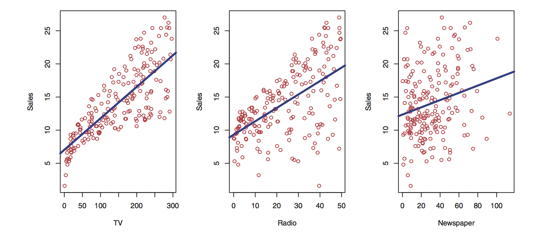
Simple model : linear regression
sales = a * radio + b * TV + c * newspaper + noise
you try to find a, b, c so that you can predict sales
- find the line closest to the points.
- minimize the distance between the line and the points.
- distance = difference between the predicted value (the points on the line) and the actual value (the real data).
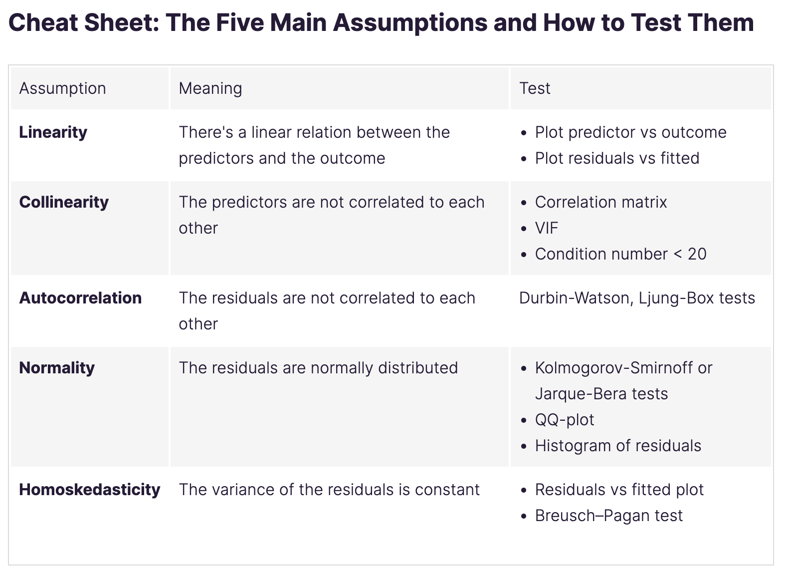
Some hypothesis needed
Heron’s method
Let’s travel back to 50 AD in ancient greece and meet Ἥρων ὁ Ἀλεξανδρεύς aka Heron of Alexandria

He invented the first steam engine (Aeolipile) and first vending machine!
And also something called Heron’s method to calculate the square root of a number. Also called for unknown reasons Babylonian method.

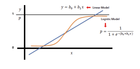
Introducing the logit / sigmoid function
- takes any number and transforms it into a number between 0 and 1

 see
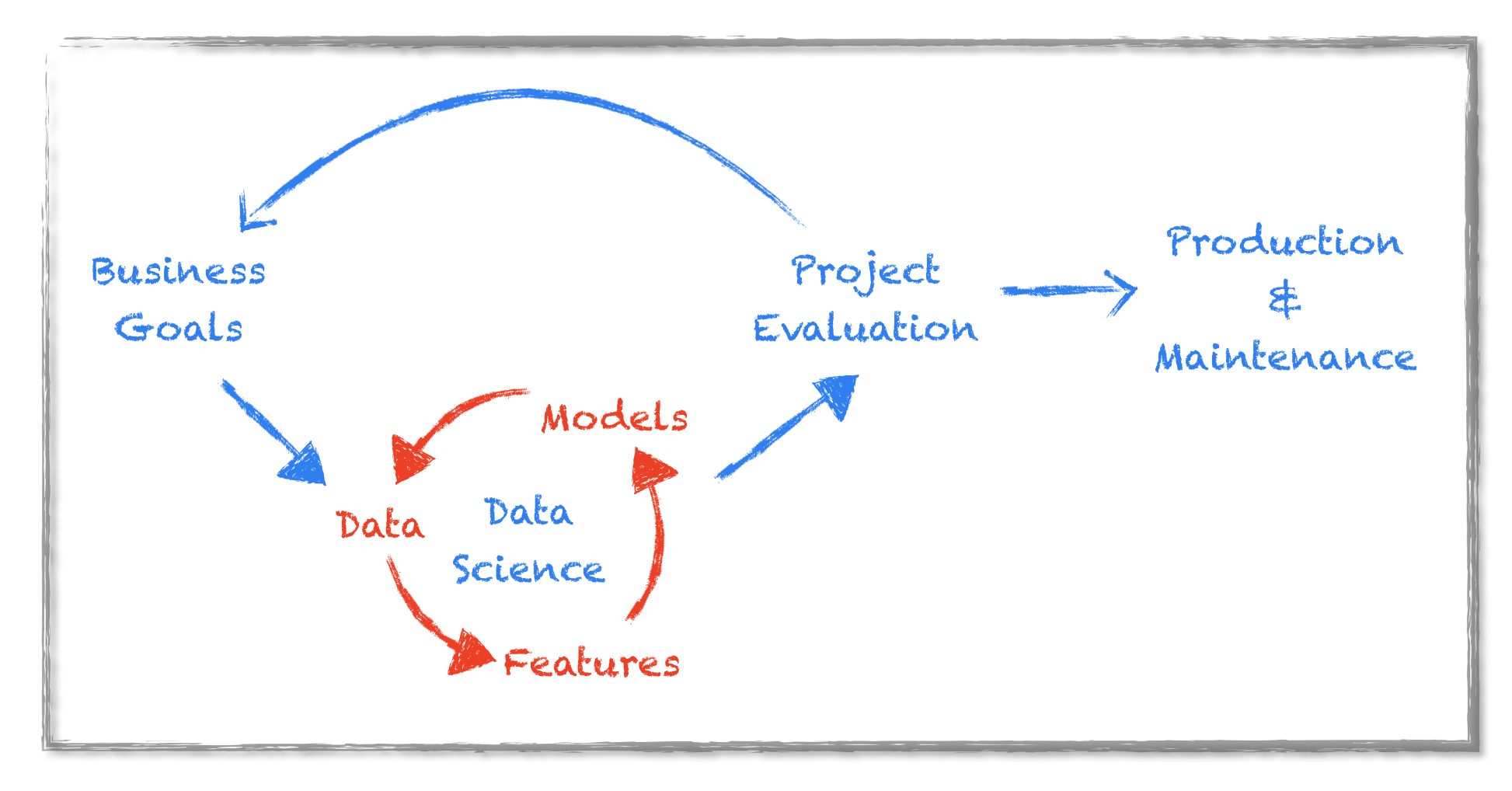
see Iterative Work process
- get the data
- clean the data
- select features based on domain knowldged
- select features automatically
- split the data into train and test
- select a model
- train the model
- evaluate the model
- back to square 1
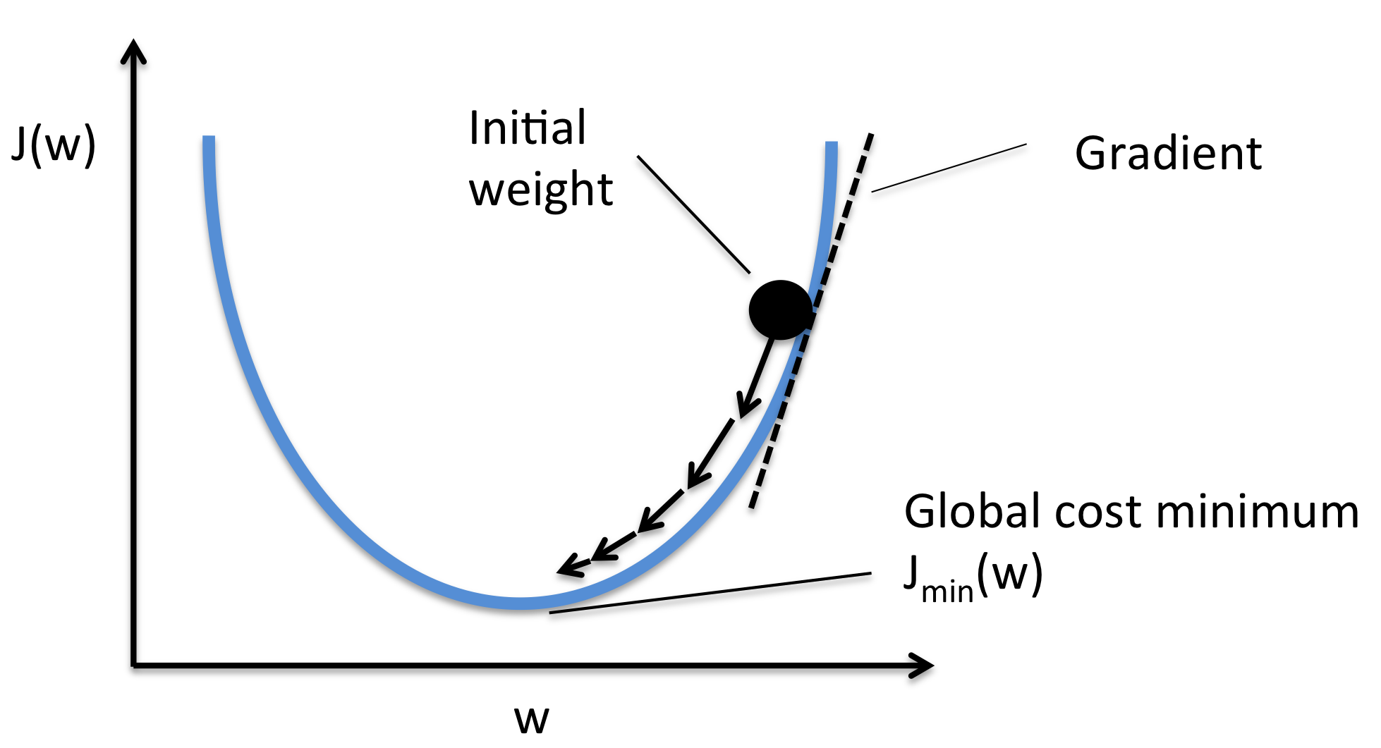
The goal of gradient descent is to find the local minima of a function.
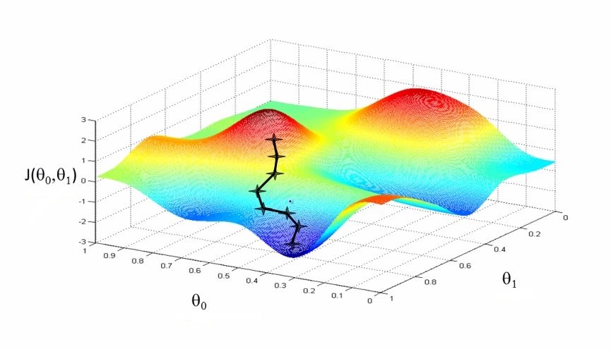
and
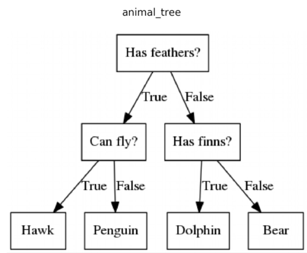
Tree based models
- decision trees
- random forests
- gradient boosting (ensembling + SGD)
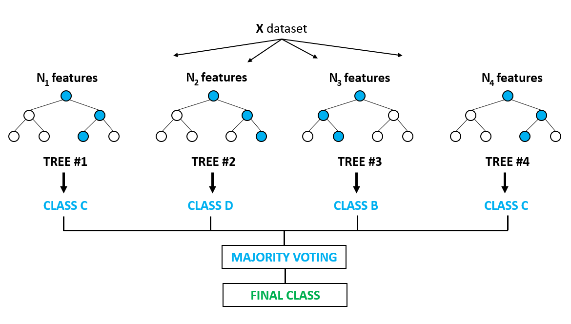
Ensembling / Bagging vs Boosting
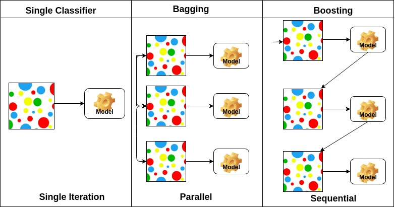
- train many weak learners or laerners that tend to overfit
- combine them to get a better model
- averaging the output : bagging
- sequentially narrowing on the errors : boosting
Overfitting and regularization
Splitting the data
You only have a set of data. You want to
- train the model => it learns the patterns in the data
- evaluate the performance of the mode with some choosen metric
But you only have a set of data.
So you split the dataset into train and test subsets
cross validation: In fact you do that multiple times with different splits and tune the model so that it performs well on average over all the splits.

This way the training data is not very different than the evaluation data. think outliers, missing values, under representation of a class etc
In the end you want your model to perform well on new unseen data.
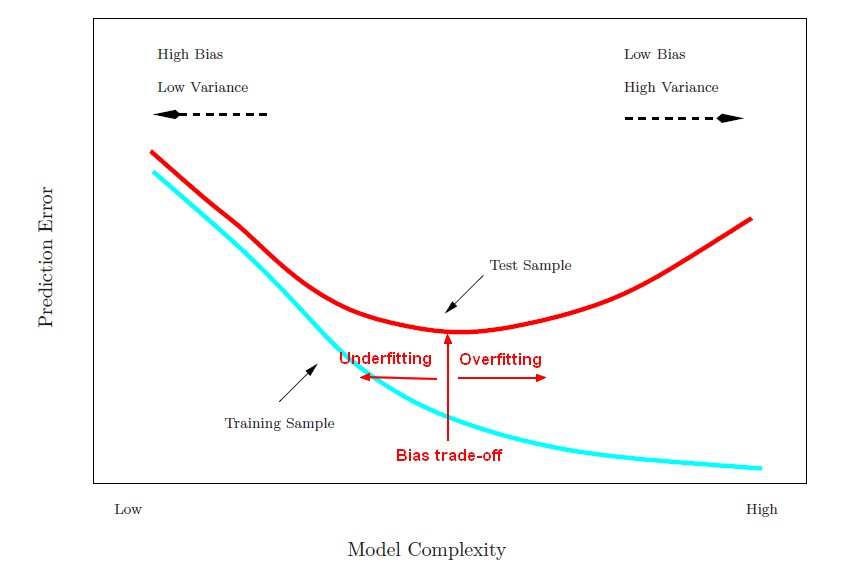
Overfitting
Overfitting is the enemy of the data scientist.
More complex models, are better at learning the training data.
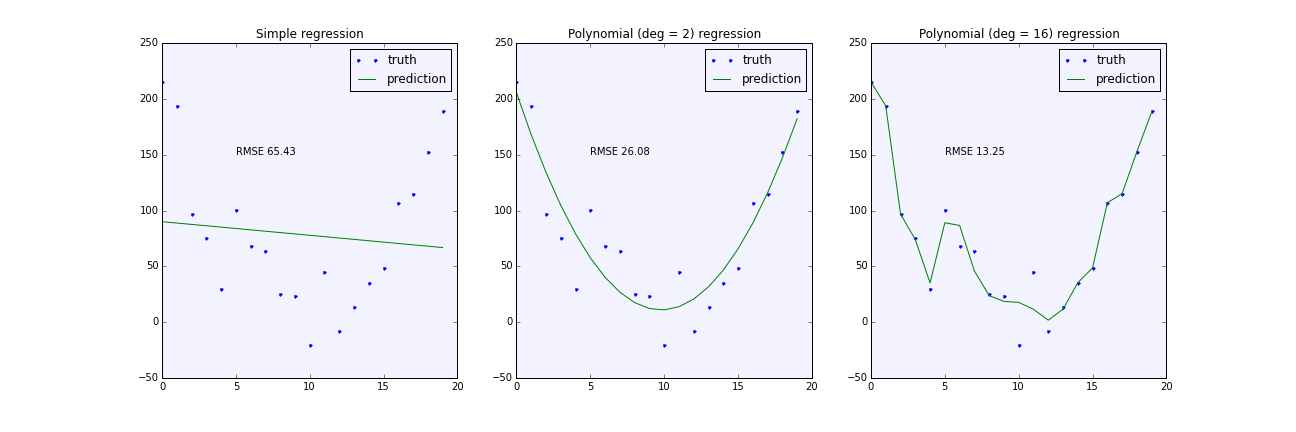
The model is so good at learning training data that it will perform great on the training data but poorly on the test data. And therefore on the real world data that it has nott seen yet.
Can’t generalize.

Detect overfit by comparing the error on the training data and the error on the test data.
if it is too high on the training data and too low on the test data, it is overfitting.
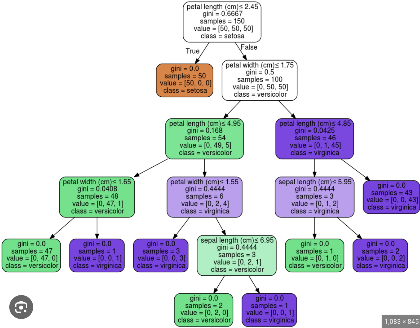
Tree pruning
This is a decision tree trained on the Iris dataset. It is overfitting.
The same tree but limited to a depth of 2
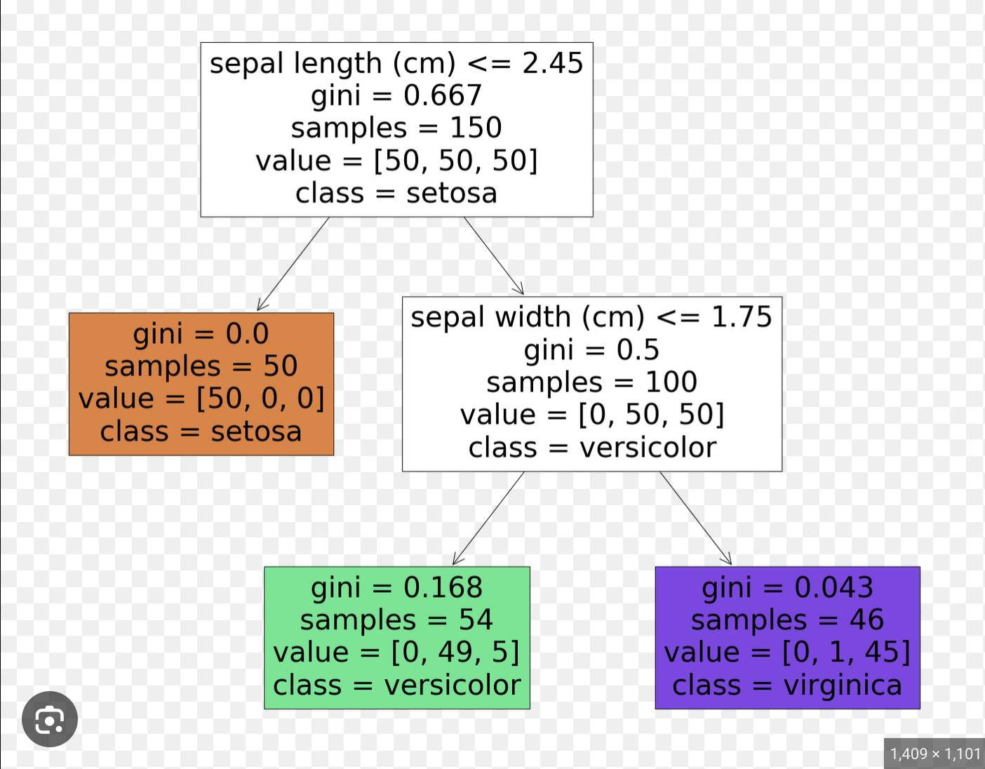
No longer overfits, but poorer performance.
So train many trees (pruned or not pruned), each on a random subset of the data. then average
You have random forests.
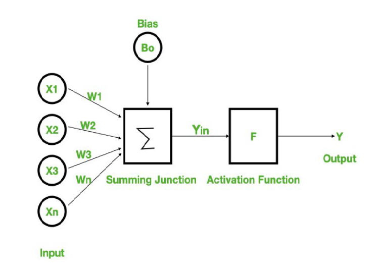
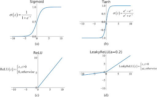
Activation function is what makes the model non linear.
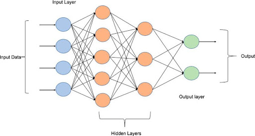
Multi layer perceptron
Single-layer perceptrons are only capable of learning linearly separable patterns
Can learn AND but not XOR
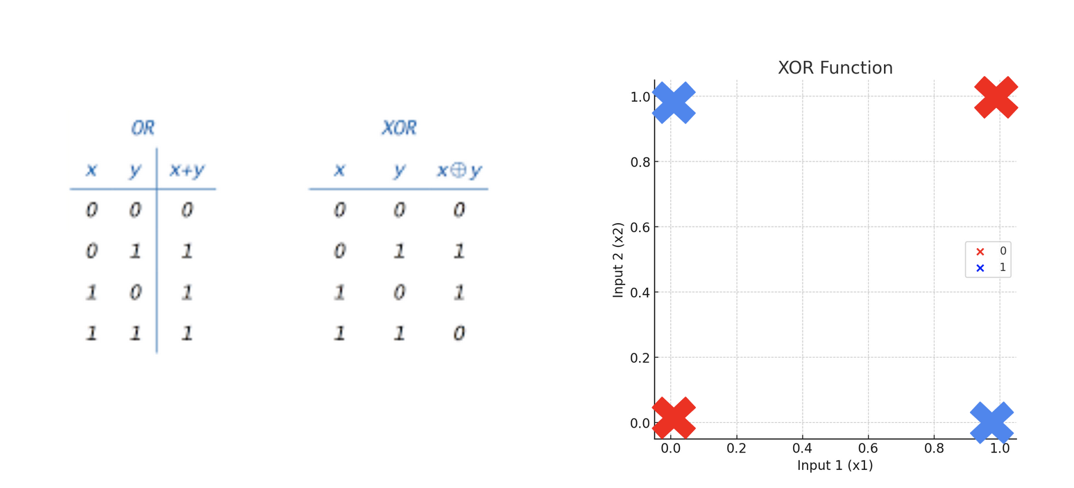
a feedforward neural network with two or more layers (also called a multilayer perceptron) had greater processing power than perceptrons with one layer (also called a single-layer perceptron). (wikipedia)
see Notebook: XOR vs AND
Regularisation for Neural Networks
On top of L2/L1 regularisation, dropout consists in randomly setting some weights to zero during training.

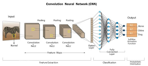
CNN : convolutional neural networks

Replace the linear regression with convolutions.
Excellent for
- images
- time series (1D)
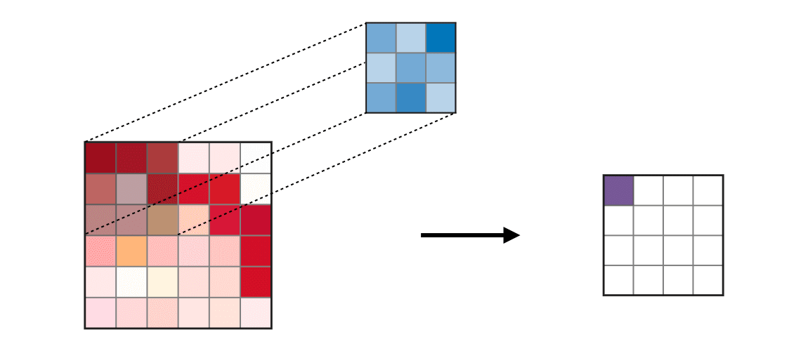
Each convolution layer extracts features from the previous layer. It zooms out and abstracts the patterns

Typical CNN
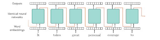
RNNs : Recurrent Neural Networks
Great for time series, NLP and any type of sequential data
Example of a more complex NN : Inception
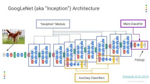
https://en.wikipedia.org/wiki/Inception_(deep_learning_architecture)
Inception[1] is a family of convolutional neural network (CNN) for computer vision, introduced by researchers at Google in 2014 as GoogLeNet
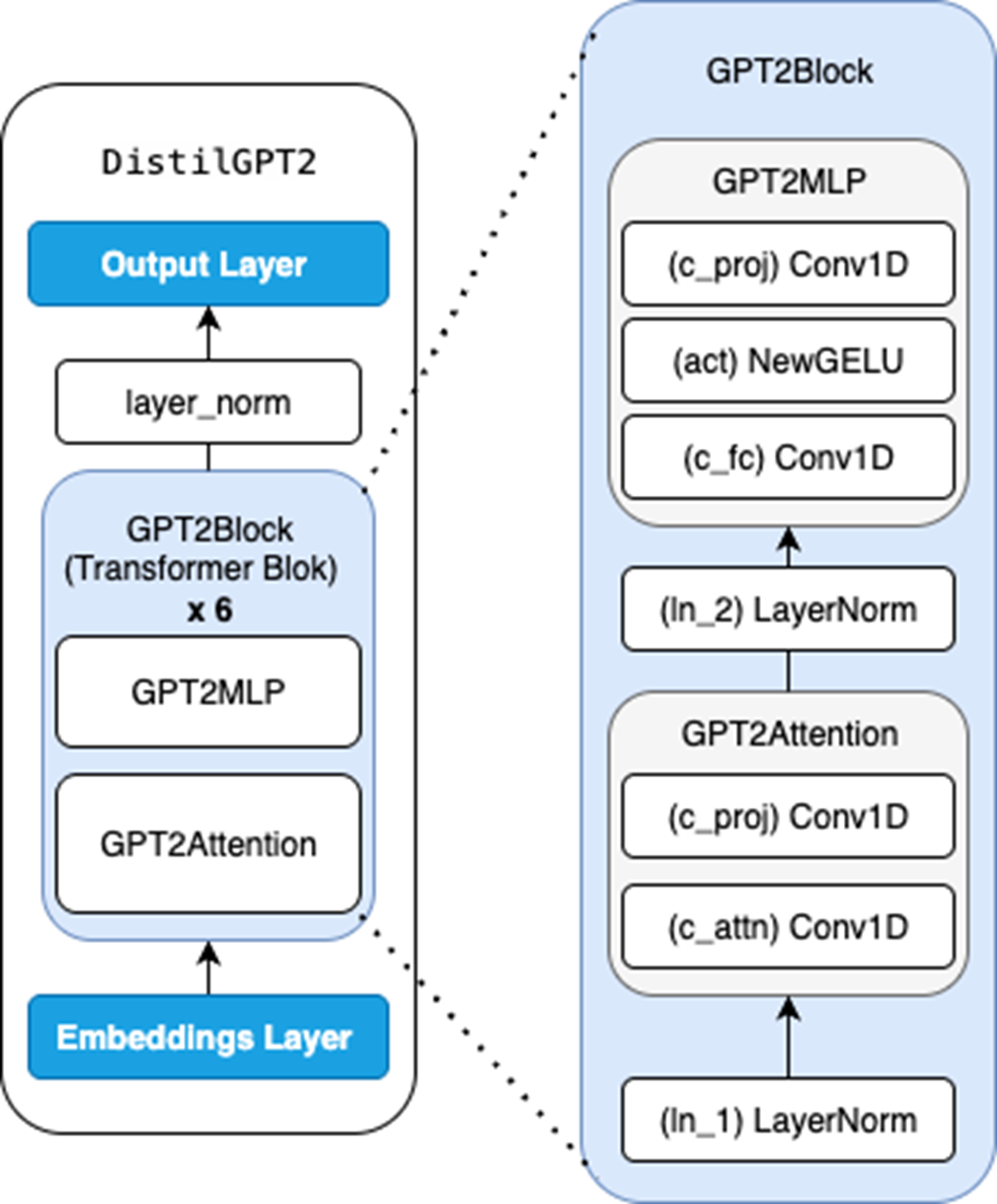
Transformers
Architecture of GPT-2